[Click here for a PDF of this post with nicer formatting]
To get a feel for how to generate the MLN equations for a circuit that has both RLC and non-linear components, consider the circuit of fig. 1.
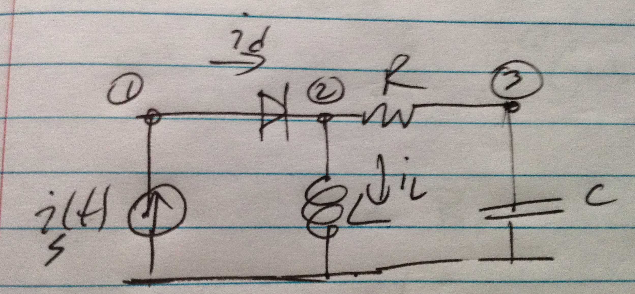
fig. 1. An RLC circuit with a diode.
The KCL equations for this circuit are
- \( 0 = i_s – i_d \)
- \( i_L + \frac{v_2 – v_3}{R} = i_d \)
- \( \frac{v_3 – v_2}{R} + C \frac{dv_3}{dt} = 0 \)
- \( -v_2 + L \frac{d i_L}{dt} = 0 \)
- \( i_d = I_0 \lr{ e^{(v_1 – v_2)/v_T} – 1} \)
FIXME: for the diode, is that the right voltage sign with respect to the current direction?
With \( Z = 1/R \), these can be put into the standard MLN matrix form as
\begin{equation}\label{eqn:diodeRLCSample:20}
\begin{bmatrix}
0 & 0 & 0 & 0 \\
0 & Z & -Z & 1 \\
0 & -Z & Z & 0 \\
0 & -1 & 0 & 0 \\
\end{bmatrix}
\begin{bmatrix}
v_1 \\
v_2 \\
v_3 \\
i_L \\
\end{bmatrix}
+
\begin{bmatrix}
0 & 0 & 0 & 0 \\
0 & 0 & 0 & 0 \\
0 & 0 & C & 0 \\
0 & 0 & 0 & L \\
\end{bmatrix}
{\begin{bmatrix}
v_1 \\
v_2 \\
v_3 \\
i_L \\
\end{bmatrix}}’
=
\begin{bmatrix}
I_0 & 1 \\
-I_0 & 0 \\
0 & 0 \\
0 & 0 \\
\end{bmatrix}
\begin{bmatrix}
1 \\
i_s(t) \\
\end{bmatrix}
+
\begin{bmatrix}
-I_0 \\
I_0 \\
0 \\
0 \\
\end{bmatrix}
\begin{bmatrix}
e^{(v_2 – v_3)/v_T}
\end{bmatrix}
\end{equation}
Let’s write this as
\begin{equation}\label{eqn:diodeRLCSample:40}
\BG \BX(t) + \BC \dot{\BX}(t) = \BB \Bu(t) + \BD \Bw(t).
\end{equation}
Here \( \Bu(t) \) collects up all the unique signature sources (for example sources with each different frequency in the system), and \( \Bw(t) \) is a vector of all the unique non-linear (time dependent) terms.
Assuming a bandwidth limited periodic source we know how to express any of the time dependent variables \( v_1, … \) in terms of their (discrete) Fourier transforms. Suppose that
the Fourier coefficients for \( v_a(t), u_b(t), w_c(t) \) are given by
\begin{equation}\label{eqn:diodeRLCSample:60}
\begin{aligned}
v_a(t) &= \sum_{n = -N}^N V_n^{(a)} e^{j \omega_0 n t} \\
u_b(t) &= \sum_{n = -N}^N U_n^{(b)} e^{j \omega_0 n t} \\
w_c(t) &= \sum_{n = -N}^N W_n^{(c)} e^{j \omega_0 n t}.
\end{aligned}
\end{equation}
For example, in this circuit, if the source was zero phase signal at the fundamental frequency of our Fourier basis (\( i_s(t) = e^{j \omega_0 t} \)), the only non-zero Fourier components \( U_n^{(a)} \) would be \( U_0^{(1)} = 1, U_1^{(2)} = 1 \).
Equation \ref{eqn:diodeRLCSample:40} then becomes
\begin{equation}\label{eqn:diodeRLCSample:80}
0 = \sum_{n=-N}^N
e^{j n \omega_0 t}
\lr{
\lr{
\BG + j \omega_0 n \BC
}
\begin{bmatrix}
V_n^{(1)} \\
V_n^{(2)} \\
\vdots
\end{bmatrix}
– \BB
\begin{bmatrix}
U_n^{(1)} \\
U_n^{(2)} \\
\end{bmatrix}
– \BD
\begin{bmatrix}
W_n^{(1)} \\
\end{bmatrix}
}
\end{equation}
The time dependence in the linear terms is nicely taken of by this transformation to the frequency domain. However, we have a fairly messy structure with sums of Fourier components instead of the nice Fourier component vectors that we see in \S A.4 of [1]. That reference does consider multivariable problems like this one, so it looks like fully digesting that methodology is the next step.
References
Giannini and Giorgio Leuzzi. Nonlinear Microwave Circuit Design. Wiley Online Library, 2004.