[Click here for a PDF of this post with nicer formatting]
Disclaimer
Peeter’s lecture notes from class. These may be incoherent and rough.
These are notes for the UofT course PHY1520, Graduate Quantum Mechanics, taught by Prof. Paramekanti, covering chap 3. content from [1].
Angular momentum (wrap up.)
We found
\begin{equation}\label{eqn:qmLecture15:20}
\begin{aligned}
\hat{\BL^2} \ket{j, m} &= j(j+1) \Hbar^2 \ket{j,m} \\
\hat{L}_z \ket{j, m} &= \Hbar m \ket{j,m} \\
\hat{L}_{\pm} \ket{j, m } &= \Hbar \sqrt{(j \mp m)(j \pm m + 1)} \ket{j, m \pm 1 }
\end{aligned}
\end{equation}
or Schwinger
\begin{equation}\label{eqn:qmLecture15:40}
\begin{aligned}
\hat{L}_z &= \inv{2} \lr{ \hat{n}_1 – \hat{n}_2 } \Hbar \\
\hat{L}_{+} &= a_1^\dagger a_2 \Hbar \\
\hat{L}_{-} &= a_1 a_2^\dagger \Hbar \\
j &= \inv{2} \lr{ \hat{n}_1 + \hat{n}_2 },
\end{aligned}
\end{equation}
where each of the \( a_1, a_2 \) operators obey
\begin{equation}\label{eqn:qmLecture15:60}
\begin{aligned}
\antisymmetric{a_1}{a_1^\dagger} &= 1 \\
\antisymmetric{a_2}{a_2^\dagger} &= 1
\end{aligned}
\end{equation}
and any pair of different index \( a \) operators commute, as in
\begin{equation}\label{eqn:qmLecture15:80}
\antisymmetric{a_1}{a_2^\dagger} = 0.
\end{equation}
Representations
It’s possible to compute matrix representations of the rotation operators
\begin{equation}\label{eqn:qmLecture15:100}
\hat{R}_\ncap(\phi) = e^{i \hat{\BL} \cdot \ncap \phi/\Hbar}.
\end{equation}
With respect to a ket it’s possible to find
\begin{equation}\label{eqn:qmLecture15:120}
e^{i \hat{\BL} \cdot \ncap \phi/\Hbar} \ket{j, m}
=
\sum_{m’} d^j_{m m’}(\ncap, \phi) \ket{ j, m’ }.
\end{equation}
This has a block diagonal form that’s sketched in fig. 1.
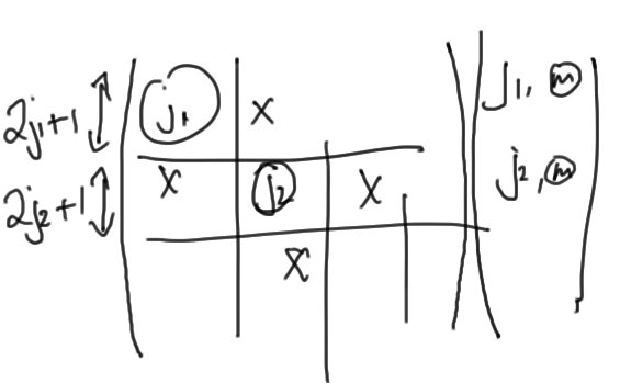
fig. 1. Block diagonal form for angular momentum matrix representation.
We can view \( d^j_{m m’}(\ncap, \phi) \) as a matrix, representing the rotation. The problem of determining these matrices can be reduced to that of determining the matrix for \( \hat{\BL} \), because once we have that we can exponentiate that.
Example: spin 1/2
From the eigenvalue relationships, with basis states
\begin{equation}\label{eqn:qmLecture15:160}
\begin{aligned}
\ket{\uparrow} &=
\begin{bmatrix}
1 \\
0
\end{bmatrix} \\
\ket{\downarrow} &=
\begin{bmatrix}
0 \\
1 \\
\end{bmatrix}
\end{aligned}
\end{equation}
we find
\begin{equation}\label{eqn:qmLecture15:180}
\begin{aligned}
\hat{L}_z &= \frac{\Hbar}{2} \begin{bmatrix} 1 & 0 \\ 0 & -1 \\ \end{bmatrix} \\
\hat{L}_{+} &= \frac{\Hbar}{2}
\begin{bmatrix}
0 & 1 \\
0 & 0
\end{bmatrix} \\
\hat{L}_{-} &= \frac{\Hbar}{2}
\begin{bmatrix}
0 & 0 \\
1 & 0
\end{bmatrix}.
\end{aligned}
\end{equation}
Rearranging we find the Pauli matrices
\begin{equation}\label{eqn:qmLecture15:200}
\hat{L}_k = \inv{2} \Hbar \sigma_i.
\end{equation}
Noting that \( \lr{ \Bsigma \cdot \ncap }^2 = 1 \), and \( \lr{\Bsigma \cdot \ncap }^3 = \Bsigma \cdot \ncap \), the rotation matrix is
\begin{equation}\label{eqn:qmLecture15:220}
e^{ i \Bsigma \cdot \ncap \phi/2 } \ket{\inv{2}, m} = \lr{ \cos( \phi/2 ) + i \Bsigma \cdot \ncap \sin(\phi/2) } \ket{\inv{2}, m}.
\end{equation}
The steps are
- Enumerate the states.
\begin{equation}\label{eqn:qmLecture15:140}
j_1 = \inv{2} \leftrightarrow\, \mbox{2 states (dimension of irrep = 2)}
\end{equation} - Construct the \( \hat{\BL} \) matrices.
- Construct \( d_{m m’}^j(\ncap, \phi) \).
Angular momentum operator in space representation
For \( L = 1 \) it turns out that the rotation matrices turn out to be the 3D rotation matrices. In the space representation
\begin{equation}\label{eqn:qmLecture15:240}
\BL = \Br \cross \Bp,
\end{equation}
the coordinates of the operator are
\begin{equation}\label{eqn:qmLecture15:260}
\hat{L}_k = i \epsilon_{k m n} r_m \lr{ -i \Hbar \PD{r_n}{} }
\end{equation}
We see that scaling \( \Br \rightarrow \alpha \Br \) does not change this operator, allowing for an angular representation \( \hat{L}_k(\theta, \phi) \) that have the form
\begin{equation}\label{eqn:qmLecture15:280}
\begin{aligned}
\hat{L}_z &= -i \Hbar \PD{\phi}{} \\
\hat{L}_{\pm} &= \Hbar \lr{ \pm \PD{\theta}{} + i \cot \theta \PD{\phi}{} }.
\end{aligned}
\end{equation}
Here \( \theta \) and \( \phi \) are the polar and azimuthal angles respectively as illustrated in fig. 2.
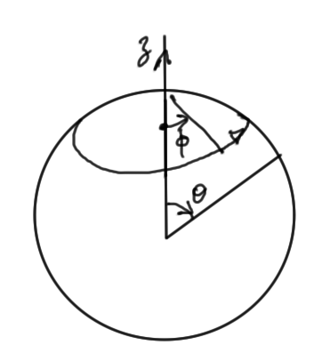
fig. 2. Spherical coordinate convention.
The equivalent wave function representation of the problem is
\begin{equation}\label{eqn:qmLecture15:300}
\begin{aligned}
\hat{\BL} Y_{lm}(\theta, \phi) &= \Hbar^2 l (l + 1) Y_{lm}(\theta, \phi) \\
\hat{L}_z Y_{lm}(\theta, \phi) &= \Hbar m Y_{lm}(\theta, \phi) \\
\end{aligned}
\end{equation}
One can find these functions
\begin{equation}\label{eqn:qmLecture15:320}
Y_{lm}(\theta, \phi) = P_{l, m}(\cos \theta) e^{i m \phi},
\end{equation}
where \( P_{l, m}(\cos \theta) \) are called the associated Legendre polynomials. This can be applied whenever we have
\begin{equation}\label{eqn:qmLecture15:340}
\antisymmetric{H}{\hat{L}_k} = 0.
\end{equation}
where all the eigenfunctions will have the form
\begin{equation}\label{eqn:qmLecture15:360}
\Psi(r, \theta, \phi) = R(r) Y_{lm}(\theta, \phi).
\end{equation}
Addition of angular momentum
Since \( \hat{\BL} \) is a vector we expect to be able to add angular momentum in some way similar to the addition of classical vectors as illustrated in fig. 3.

fig. 3. Classical vector addition.
When we have a potential that depends only on the difference in position \( V(\Br_1 – \Br_2) \) then we know from classical problems it is effective to work in center of mass coordinates
\begin{equation}\label{eqn:qmLecture15:380}
\begin{aligned}
\hat{\BR}_{\textrm{cm}} &= \frac{\hat{\Br}_1 + \hat{\Br}_2}{2} \\
\hat{\BP}_{\textrm{cm}} &= \hat{\Bp}_1 + \hat{\Bp}_2
\end{aligned}
\end{equation}
where
\begin{equation}\label{eqn:qmLecture15:400}
\antisymmetric{\hat{R}_i}{\hat{P}_j} = i \Hbar \delta_{ij}.
\end{equation}
Given
\begin{equation}\label{eqn:qmLecture15:420}
\hat{\BL}_1 + \hat{\BL}_2 = \hat{\BL}_{\textrm{tot}},
\end{equation}
do we have
\begin{equation}\label{eqn:qmLecture15:440}
\antisymmetric{
\hat{L}_{\textrm{tot}, i}
}{
\hat{L}_{\textrm{tot}, j}
}
= i \Hbar \epsilon_{i j k} \hat{L}_{\textrm{tot}, k} ?
\end{equation}
That is
\begin{equation}\label{eqn:qmLecture15:460}
\antisymmetric{\hat{L}_{1,i} + \hat{L}_{1,j}}{\hat{L}_{2,i} + \hat{L}_{2,j}} = i \Hbar \epsilon_{i j k} \lr{ \hat{L}_{1,k} + \hat{L}_{1,k} }
\end{equation}
FIXME: Right at the end of the lecture, there was a mention of something about whether or not \( \hat{\BL}_1^2 \) and \( \hat{L}_{1,z} \) were sharply defined, but I missed it. Ask about this if not covered in the next lecture.
References
[1] Jun John Sakurai and Jim J Napolitano. Modern quantum mechanics. Pearson Higher Ed, 2014.