[Click here for a PDF of this post with nicer formatting]
Disclaimer
Peeter’s lecture notes from class. These may be incoherent and rough.
These are notes for the UofT course PHY1520, Graduate Quantum Mechanics, taught by Prof. Paramekanti, covering \textchapref{{5}} [1] content.
Variational method
Today we want to use the variational degree of freedom to try to solve some problems that we don’t have analytic solutions for.
Anharmonic oscillator
\begin{equation}\label{eqn:qmLecture19:20}
V(x) = \inv{2} m \omega^2 x^2 + \lambda x^4, \qquad \lambda \ge 0.
\end{equation}
With the potential growing faster than the harmonic oscillator, which had a ground state solution
\begin{equation}\label{eqn:qmLecture19:40}
\psi(x) = \inv{\pi^{1/4}} \inv{a_0^{1/2} } e^{- x^2/2 a_0^2},
\end{equation}
where
\begin{equation}\label{eqn:qmLecture19:60}
a_0 = \sqrt{\frac{\Hbar}{m \omega}}.
\end{equation}
Let’s try allowing \( a_0 \rightarrow a \), to be a variational degree of freedom
\begin{equation}\label{eqn:qmLecture19:80}
\psi_a(x) = \inv{\pi^{1/4}} \inv{a^{1/2} } e^{- x^2/2 a^2},
\end{equation}
\begin{equation}\label{eqn:qmLecture19:100}
\bra{\psi_a} H \ket{\psi_a}
=
\bra{\psi_a} \frac{p^2}{2m} + \inv{2} m \omega^2 x^2 + \lambda x^4 \ket{\psi_a}
\end{equation}
We can find
\begin{equation}\label{eqn:qmLecture19:120}
\expectation{x^2} = \inv{2} a^2
\end{equation}
\begin{equation}\label{eqn:qmLecture19:140}
\expectation{x^4} = \frac{3}{4} a^4
\end{equation}
Define
\begin{equation}\label{eqn:qmLecture19:160}
\tilde{\omega} = \frac{\Hbar}{m a^2},
\end{equation}
so that
\begin{equation}\label{eqn:qmLecture19:180}
\overline{{E}}_a
=
\bra{\psi_a} \lr{ \frac{p^2}{2m} + \inv{2} m \tilde{\omega}^2 x^2 }
+ \lr{
\inv{2} m \lr{ \omega^2 – \tilde{\omega}^2 } x^2
+
\lambda x^4 }
\ket{\psi_a}
=
\inv{2} \Hbar \tilde{\omega} + \inv{2} m \lr{ \omega^2 – \tilde{\omega}^2 } \inv{2} a^2 + \frac{3}{4} \lambda a^4.
\end{equation}
Write this as
\begin{equation}\label{eqn:qmLecture19:200}
\overline{{E}}_{\tilde{\omega}}
=
\inv{2} \Hbar \tilde{\omega} + \inv{4} \frac{\Hbar}{\tilde{\omega}} \lr{ \omega^2 – \tilde{\omega}^2 } + \frac{3}{4} \lambda \frac{\Hbar^2}{m^2 \tilde{\omega}^2 }.
\end{equation}
This might look something like fig. 1.
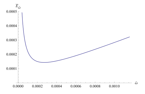
fig. 1: Energy after perturbation.
Demand that
\begin{equation}\label{eqn:qmLecture19:220}
0
= \PD{\tilde{\omega}}{ \overline{{E}}_{\tilde{\omega}}}
=
\frac{\Hbar}{2} – \frac{\Hbar}{4} \frac{\omega^2}{\tilde{\omega}^2}
– \frac{\Hbar}{4}
+ \frac{3}{4} (-2) \frac{\lambda \Hbar^2}{m^2 \tilde{\omega}^3}
=
\frac{\Hbar}{4}
\lr{
1 – \frac{\omega^2}{\tilde{\omega}^2}
– 6 \frac{\lambda \Hbar}{m^2 \tilde{\omega}^3}
}
\end{equation}
or
\begin{equation}\label{eqn:qmLecture19:260}
\tilde{\omega}^3 – \omega^2 \tilde{\omega} – \frac{6 \lambda \Hbar}{m^2} = 0.
\end{equation}
for \( \lambda a_0^4 \ll \Hbar \omega \), we have something like \( \tilde{\omega} = \omega + \epsilon \). Expanding \ref{eqn:qmLecture19:260} to first order in \( \epsilon \), this gives
\begin{equation}\label{eqn:qmLecture19:280}
\omega^3 + 3 \omega^2 \epsilon – \omega^2 \lr{ \omega + \epsilon } – \frac{6 \lambda \Hbar}{m^2} = 0,
\end{equation}
so that
\begin{equation}\label{eqn:qmLecture19:300}
2 \omega^2 \epsilon = \frac{6 \lambda \Hbar}{m^2},
\end{equation}
and
\begin{equation}\label{eqn:qmLecture19:320}
\Hbar \epsilon = \frac{ 3 \lambda \Hbar^2}{m^2 \omega^2 } = 3 \lambda a_0^4.
\end{equation}
Plugging into
\begin{equation}\label{eqn:qmLecture19:340}
\overline{{E}}_{\omega + \epsilon}
=
\inv{2} \Hbar \lr{ \omega + \epsilon }
+ \inv{4} \frac{\Hbar}{\omega} \lr{ -2 \omega \epsilon + \epsilon^2 } + \frac{3}{4} \lambda \frac{\Hbar^2}{m^2 \omega^2 }
\approx
\inv{2} \Hbar \lr{ \omega + \epsilon }
– \inv{2} \Hbar \epsilon
+ \frac{3}{4} \lambda \frac{\Hbar^2}{m^2 \omega^2 }
=
\inv{2} \Hbar \omega + \frac{3}{4} \lambda a_0^4.
\end{equation}
With \ref{eqn:qmLecture19:320}, that is
\begin{equation}\label{eqn:qmLecture19:540}
\overline{{E}}_{\tilde{\omega} = \omega + \epsilon} \approx \inv{2} \Hbar \lr{ \omega + \frac{\epsilon}{2} }.
\end{equation}
The energy levels are shifted slightly for each shift in the Hamiltonian frequency.
What do we have in the extreme anharmonic limit, where \( \lambda a_0^4 \gg \Hbar \omega \). Now we get
\begin{equation}\label{eqn:qmLecture19:360}
\tilde{\omega}^\conj = \lr{ \frac{ 6 \Hbar \lambda }{m^2} }^{1/3},
\end{equation}
and
\begin{equation}\label{eqn:qmLecture19:380}
\overline{{E}}_{\tilde{\omega}^\conj} = \frac{\Hbar^{4/3} \lambda^{1/3}}{m^{2/3}} \frac{3}{8} 6^{1/3}.
\end{equation}
(this last result is pulled from a web treatment somewhere of the anharmonic oscillator). Note that the first factor in this energy, with \( \Hbar^4 \lambda/m^2 \) traveling together could have been worked out on dimensional grounds.
This variational method tends to work quite well in these limits. For a system where \( m = \omega = \Hbar = 1 \), for this problem, we have
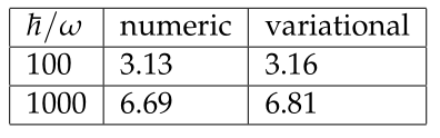
tab. 1: Comparing numeric and variational solutions.
Example: (sketch) double well potential
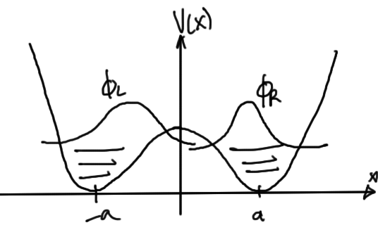
fig. 2: Double well potential.
\begin{equation}\label{eqn:qmLecture19:400}
V(x) = \frac{m \omega^2}{8 a^2} \lr{ x – a }^2\lr{ x + a}^2.
\end{equation}
Note that this potential, and the Hamiltonian, both commute with parity.
We are interested in the regime where \( a_0^2 = \frac{\Hbar}{m \omega} \ll a^2 \).
Near \( x = \pm a \), this will be approximately
\begin{equation}\label{eqn:qmLecture19:420}
V(x) = \inv{2} m \omega^2 \lr{ x \pm a }^2.
\end{equation}
Guessing a wave function that is an eigenstate of parity
\begin{equation}\label{eqn:qmLecture19:440}
\Psi_{\pm} = g_{\pm} \lr{ \phi_{\textrm{R}}(x) \pm \phi_{\textrm{L}}(x) }.
\end{equation}
perhaps looking like the even and odd functions sketched in fig. 3, and fig. 4.
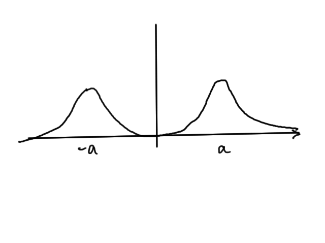
fig. 3. Even double well function
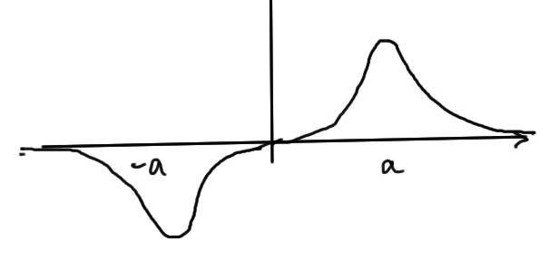
fig. 4. Odd double well function
Using harmonic oscillator functions
\begin{equation}\label{eqn:qmLecture19:460}
\begin{aligned}
\phi_{\textrm{L}}(x) &= \Psi_{{\textrm{H}}.{\textrm{O}}.}(x + a) \\
\phi_{\textrm{R}}(x) &= \Psi_{{\textrm{H}}.{\textrm{O}}.}(x – a)
\end{aligned}
\end{equation}
After doing a lot of integral (i.e. in the problem set), we will see a splitting of the variational energy levels as sketched in fig. 5.
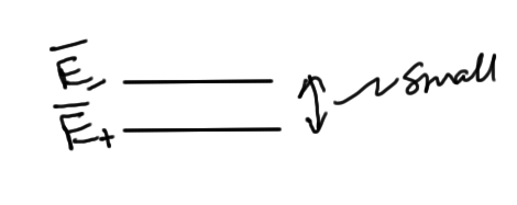
fig. 5. Splitting for double well potential.
This sort of level splitting was what was used in the very first mazers.
Perturbation theory (outline)
Given
\begin{equation}\label{eqn:qmLecture19:480}
H = H_0 + \lambda V,
\end{equation}
where \( \lambda V \) is “small”. We want to figure out the eigenvalues and eigenstates of this Hamiltonian
\begin{equation}\label{eqn:qmLecture19:500}
H \ket{n} = E_n \ket{n}.
\end{equation}
We don’t know what these are, but do know that
\begin{equation}\label{eqn:qmLecture19:520}
H_0 \ket{n^{(0)}} = E_n^{(0)} \ket{n^{(0)}}.
\end{equation}
We are hoping that the level transitions have adiabatic transitions between the original and perturbed levels as sketched in fig. 6.
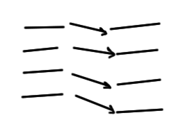
fig. 6. Adiabatic transitions.
and not crossed level transitions as sketched in fig. 7.
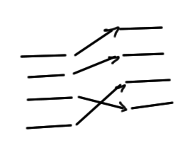
fig. 7. Crossed level transitions.
If we have level crossings (which can in general occur), as opposed to adiabatic transitions, then we have no hope of using perturbation theory.
References
[1] Jun John Sakurai and Jim J Napolitano. Modern quantum mechanics. Pearson Higher Ed, 2014.