Month: October 2018

PHY2403H Quantum Field Theory. Lecture 12: Klein-Gordon Green’s function, Feynman propagator path deformation, Weightmann function, Retarded Green’s function. Taught by Prof. Erich Poppitz

October 22, 2018 phy2403 , , ,

[Click here for a PDF of this post with nicer formatting]

DISCLAIMER: Very rough notes from class, with some additional side notes.

These are notes for the UofT course PHY2403H, Quantum Field Theory, taught by Prof. Erich Poppitz, fall 2018.

Green’s functions for the forced Klein-Gordon equation.

The problem were were preparing to do was to study the problem of “particle creation by external classical source”.

We continue with a real scalar field, free, massive, but with an interaction with a source
\begin{equation}\label{eqn:qftLecture12:20}
S_{\text{int}} = \int d^4 x j(x) \phi(x).
\end{equation}

Modern application:

think of \( \phi \) has some SM field and think of \( j \) as due to inflaton (i.e. cosmological inflation interaction) oscillation. In the inflationary model, the process of “reheating” creates all the matter in the universe. We won’t be talking about inflation, but will be considering a toy model that has some similar characteristics to the inflationary theory.

The equation of motion that we end up with is
\begin{equation}\label{eqn:qftLecture12:40}
\lr{ \partial_\mu \partial^\mu + m^2} \phi = j,
\end{equation}
and we wish to solve this using Green’s function techniques.

Definition: Klein-Gordon Green’s function.

The QFT conventions for the Klein-Gordon Green’s function is
\begin{equation*}
\lr{ \partial_\mu \partial^\mu + m^2} G(x – y) = -i \delta^4(x – y).
\end{equation*}

As usual, we assume that it is possible to find a solution \( \phi \) by convolution
\begin{equation}\label{eqn:qftLecture12:80}
\phi(x) = i \int d^4 y G(x – y) j(y).
\end{equation}

Check:

\begin{equation}\label{eqn:qftLecture12:100}
\begin{aligned}
\lr{ \partial_\mu \partial^\mu + m^2} \phi(x)
&=
i
\lr{ \partial_\mu \partial^\mu + m^2}
\int d^4 y G(x – y) j(y) \\
&=
i \int d^4 y (-i) \delta^4(x – y) j(y) \\
&= j(x).
\end{aligned}
\end{equation}

Also, as usual, we take out our Fourier transforms, the power tool of physics, and determine the structure of the Green’s function by inverting the transform equation
\begin{equation}\label{eqn:qftLecture12:120}
G(x – y) = \int \frac{d^4 p}{(2 \pi)^4} e^{-i p \cdot (x-y) } \tilde{G}(p).
\end{equation}
Operating with KG gives
\begin{equation}\label{eqn:qftLecture12:520}
\lr{ \partial_\mu \partial^\mu + m^2}
G(x)
=
\int \frac{d^4 p}{(2 \pi)^4}
\lr{ (-i p_\mu)(-i p^\mu) + m^2 }
e^{-i p \cdot (x-y) } \tilde{G}(p).
\end{equation}
This must equal
\begin{equation}\label{eqn:qftLecture12:140}
-i \delta^4(x – y) =
-i \int \frac{d^4 p}{(2 \pi)^4} e^{-i p \cdot (x -y)},
\end{equation}
or
\begin{equation}\label{eqn:qftLecture12:160}
\lr{ m^2 – p_\mu p^\mu } \tilde{G}(p) = -i.
\end{equation}
The Green’s function in the momentum domain is
\begin{equation}\label{eqn:qftLecture12:180}
\tilde{G}(p) = \frac{i}{p^2 – m^2}.
\end{equation}

The inverse transform provides the spatial domain representation of the Green’s function
\begin{equation}\label{eqn:qftLecture12:200}
\begin{aligned}
G(x)
&=
\int \frac{d^4 p}{(2 \pi)^4} e^{-i p \cdot x }
\frac{i}{(p^0)^2 – \Bp^2 – m^2} \\
&=
\int \frac{d^3 p}{(2\pi)^3} e^{i \Bp \cdot \Bx}
\int \frac{d p_0}{2 \pi} e^{-i p_0 x^0 }
\frac{i}{(p_0 – \omega_\Bp)(p_0 + \omega_\Bp)}.
\end{aligned}
\end{equation}

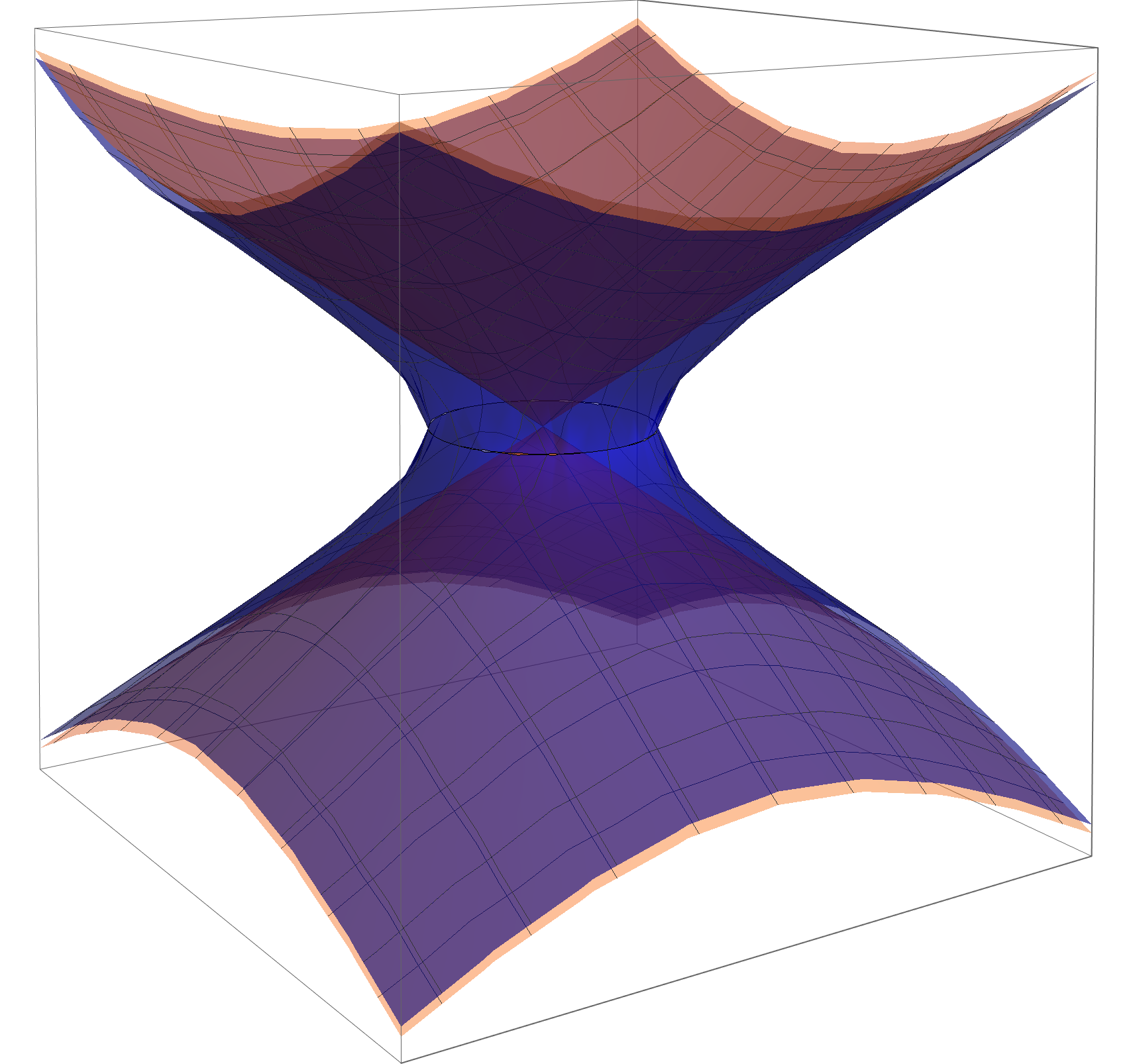
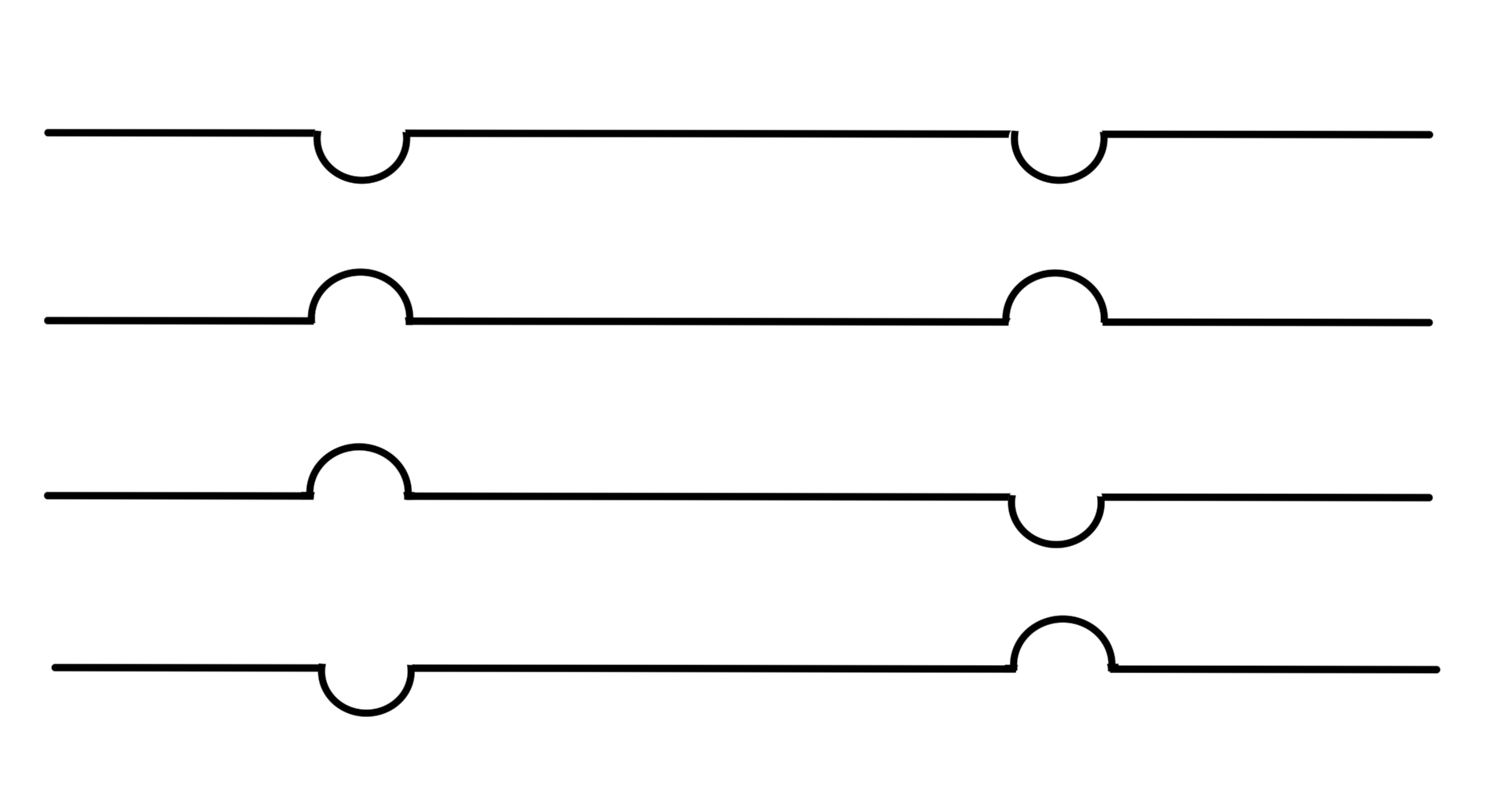
In the \( p_0 \) plane, we have two poles at \( p_0 = \pm \omega_\Bp \). There are 4 ways to go around the poles, the retarded time deformation that we used to derive the Green’s function for the harmonic oscillator, as sketched in fig. 1, the advanced time deformation sketched in fig. 2, and mixed deformations.

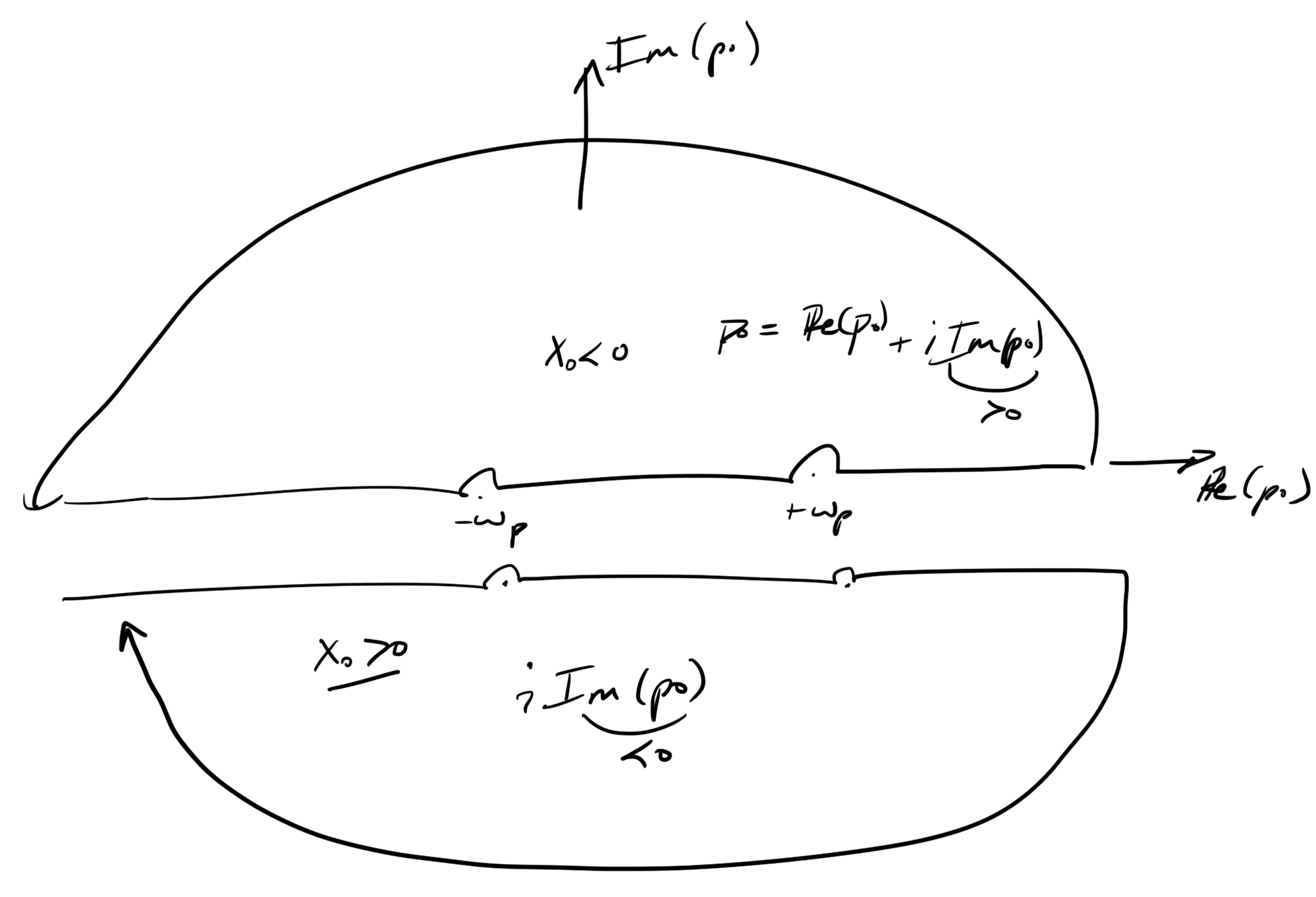
fig. 1. Retarded time deformations and contours.

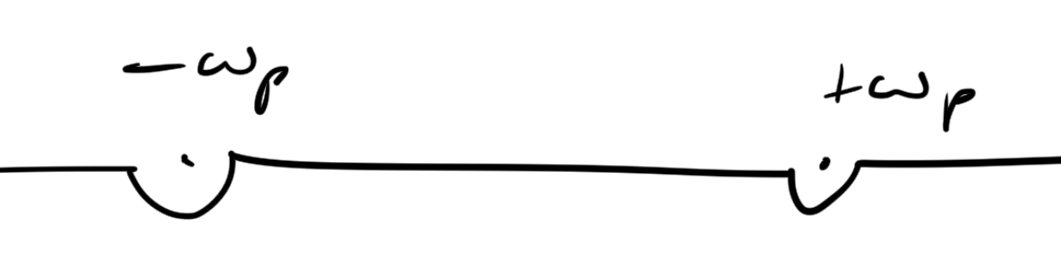
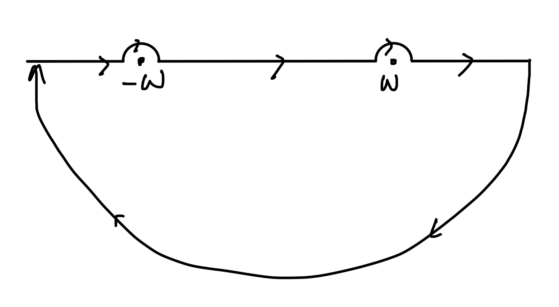
fig. 2. Advanced time deformation.

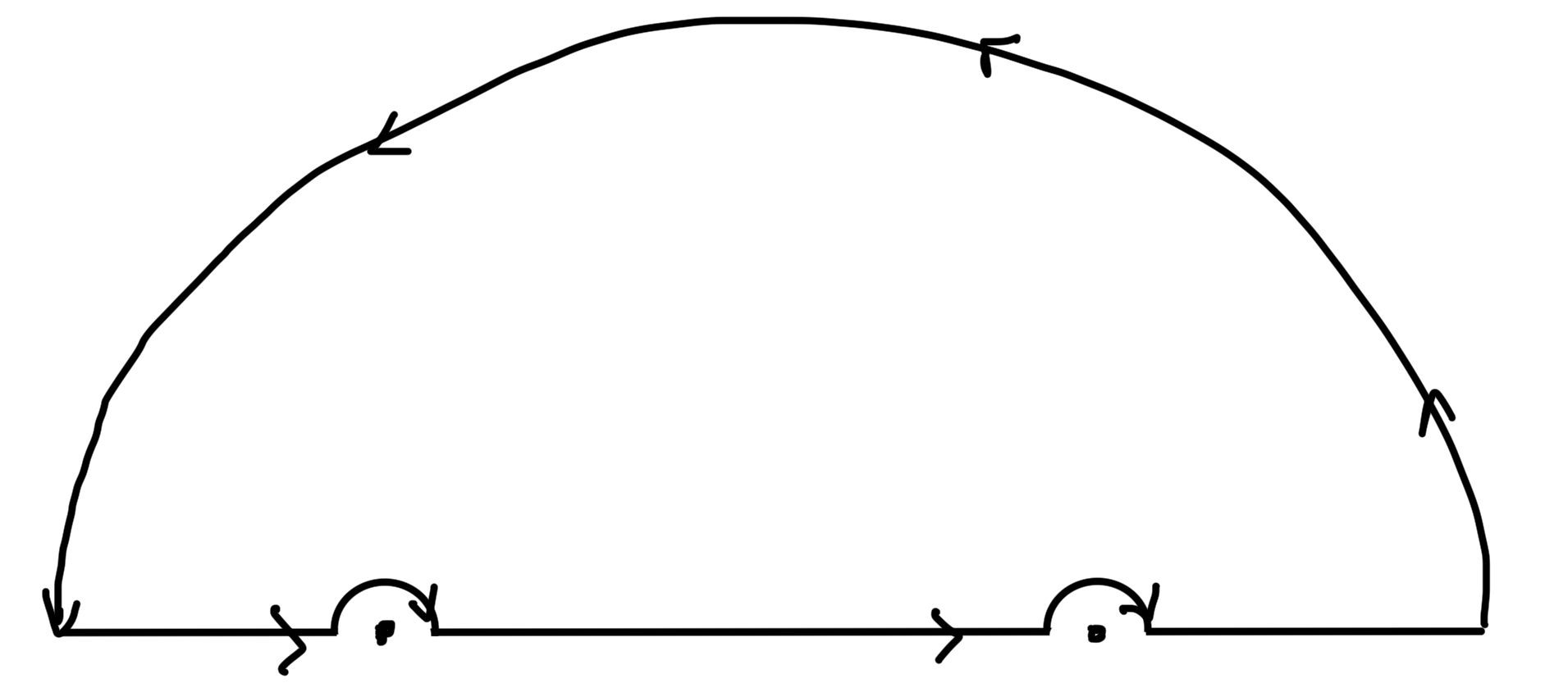
We will evaluate the integral using the “Feynman propagator” contour sketched in fig. 3. Why we use the Feynman contour, and not the retarded contour can be justified by how well this works for the perturbation methods that will be developed later.

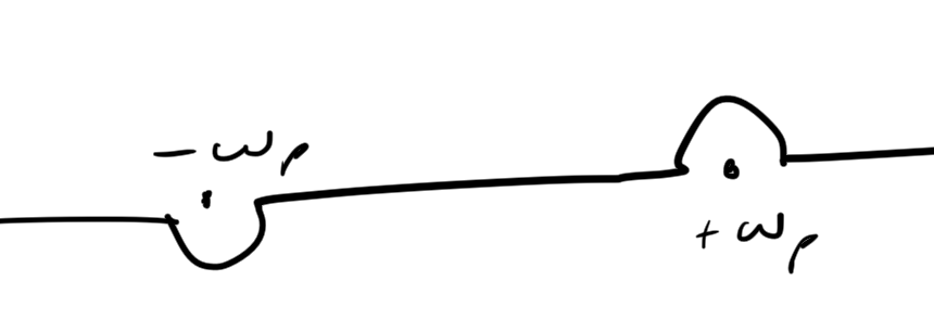
fig. 3. Feynman propagator deformation path.

Consider each contour in turn.

Case I. \( x^0 > 0 \)

For this case, we use the lower half plane contour sketched in fig. 4, which vanishes for \( \Im(p_0) < 0, x_0 > 0 \), where \( -i (i \Im(p_0) x_0) < 0 \).

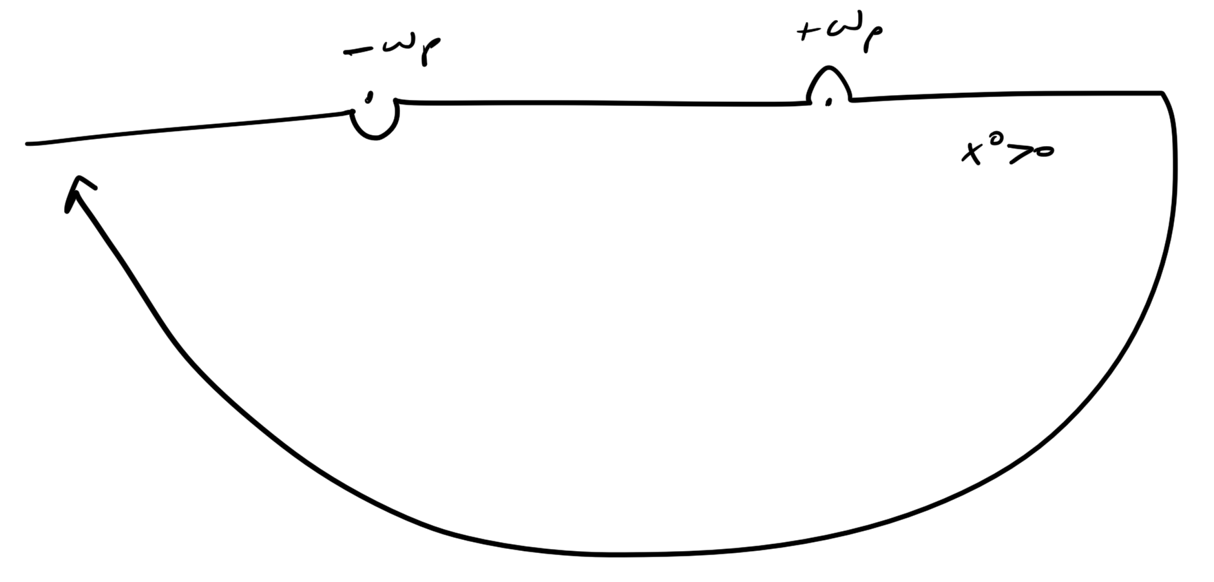
fig. 4. Feynman propagator contour for t > 0.

Here we pick up just the pole at \( p_0 = \omega_\Bp \), and take a negatively oriented path
\begin{equation}\label{eqn:qftLecture12:220}
\begin{aligned}
G_\txtF
&=
\int \frac{d^3 p}{(2\pi)^3} e^{i \Bp \cdot \Bx}
\int \frac{d p_0}{2 \pi} e^{-i p_0 x^0 }
\frac{i}{(p_0 – \omega_\Bp)(p_0 + \omega_\Bp)} \\
&=
\int \frac{d^3 p}{(2\pi)^3} e^{i \Bp \cdot \Bx}
(-2 \pi i)
\evalbar{\lr{ \frac{e^{-i p_0 x^0 }}{2 \pi}
\frac{i}{p_0 + \omega_\Bp} }}{p_0 = \omega_p} \\
&=
\int \frac{d^3 p}{(2\pi)^3} e^{i \Bp \cdot \Bx}
\frac{-2 \pi i}{2 \pi} \frac{i e^{-i p_0 x^0 } }{2 \omega_\Bp} \\
&=
\int \frac{d^3 p}{(2\pi)^3} e^{i \Bp \cdot \Bx}
\frac{ e^{-i \omega_\Bp x^0 } }{2 \omega_\Bp}.
\end{aligned}
\end{equation}

Case II. \( x^0 < 0 \)

For \( x^0 < 0 \) we use an upper half plane contour with the same deformation around the poles. This time

\begin{equation}\label{eqn:qftLecture12:240}
\begin{aligned}
G_\txtF
&=
\int \frac{d^3 p}{(2\pi)^3} e^{i \Bp \cdot \Bx}
\int \frac{d p_0}{2 \pi} e^{-i p_0 x^0 }
\frac{i}{(p_0 – \omega_\Bp)(p_0 + \omega_\Bp)} \\
&=
\int \frac{d^3 p}{(2\pi)^3} e^{i \Bp \cdot \Bx}
(+ 2 \pi i)
\evalbar{\lr{\frac{e^{-i p_0 x^0 }}{2 \pi}
\frac{i}{p_0 – \omega_\Bp}}}{p_0 = -\omega_\Bp} \\
&=
\int \frac{d^3 p}{(2\pi)^3} e^{i \Bp \cdot \Bx}
\frac{+2 \pi i}{2 \pi} \frac{i e^{-i p_0 x^0 } }{-2 \omega_\Bp} \\
&=
\int \frac{d^3 p}{(2\pi)^3} e^{i \Bp \cdot \Bx}
\frac{ e^{i \omega_\Bp x^0 } }{2 \omega_\Bp}.
\end{aligned}
\end{equation}
We’ve obtained a piecewise representation of the Green’s function, where the only difference is the sign of the \( i \omega_\Bp x^0 \) exponential.

We can combine \ref{eqn:qftLecture12:220} \ref{eqn:qftLecture12:240} by using \( \Theta \) functions
\begin{equation}\label{eqn:qftLecture12:260}
\int \frac{d^3 p}{(2\pi)^3 2 \omega_\Bp} e^{i \Bp \cdot \Bx}
\lr{
e^{-i \omega_\Bp x^0 } \Theta(x_0)
+
e^{i \omega_\Bp x^0 } \Theta(-x_0)
}.
\end{equation}
The first integral (without the \(\Theta\) factor) is the Weightmann function
\begin{equation}\label{eqn:qftLecture12:280}
D(x)
=
\int \frac{d^3 p}{(2\pi)^3 2 \omega_\Bp} \evalbar{e^{-i p \cdot x}}{p^0 = \omega_\Bp}.
\end{equation}

For the second integral, we make a change of variables \( \Bp \rightarrow -\Bp \) leaving
\begin{equation}\label{eqn:qftLecture12:300}
\begin{aligned}
\int \frac{d^3 p}{(2\pi)^3 2 \omega_\Bp} e^{i \Bp \cdot \Bx + i \omega_\Bp x^0}
&\rightarrow
\int \frac{d^3 p}{(2\pi)^3 2 \omega_\Bp} e^{-i \Bp \cdot \Bx + i \omega_\Bp x^0} \\
&=
\int \frac{d^3 p}{(2\pi)^3 2 \omega_\Bp} e^{-i p \cdot x} \\
&= D(-x),
\end{aligned}
\end{equation}
so
\begin{equation}\label{eqn:qftLecture12:340}
\boxed{
G_\txtF (x) = \Theta(x^0) D(x) + \Theta(-x^0) D(-x)
}
\end{equation}

Matrix element representation of the Weightmann function.

Recall that the Weightmann function also had a matrix element representation
\begin{equation}\label{eqn:qftLecture12:360}
D(x) = \bra{0} \phi(x) \phi(0) \ket{0}.
\end{equation}
This can be shown by expansion.
\begin{equation}\label{eqn:qftLecture12:380}
\bra{0} \phi(x) \phi(0) \ket{0}
=
\bra{0}
\int \frac{d^3 p}{(2 \pi)^3} \inv{\sqrt{2 \omega_\Bp}} \evalbar{\lr{ a_\Bp e^{-i p \cdot x} + a_\Bp^\dagger e^{i p \cdot x} }}{p_0 = \omega_\Bp}
\int \frac{d^3 q}{(2 \pi)^3} \inv{\sqrt{2 \omega_\Bq}} \lr{ a_\Bq^\dagger + a_\Bq }
\ket{0}
\end{equation}
Since \( a_\Bq \ket{0} = 0 = \bra{0} a_\Bp^\dagger \), \ref{eqn:qftLecture12:380}
reduces to
\begin{equation}\label{eqn:qftLecture12:540}
\begin{aligned}
\bra{0} \phi(x) \phi(0) \ket{0}
&=
\bra{0}
\int
\frac{d^3 p}{(2 \pi)^3}
\frac{d^3 q}{(2 \pi)^3}
\inv{\sqrt{2 \omega_\Bp}}
\inv{\sqrt{2 \omega_\Bq}}
\evalbar{\lr{ a_\Bp a_\Bq^\dagger e^{-i p \cdot x} }}{p_0 = \omega_\Bp}
\ket{0} \\
&=
\bra{0}
\int
\frac{d^3 p}{(2 \pi)^3}
\frac{d^3 q}{(2 \pi)^3}
\inv{\sqrt{2 \omega_\Bp}}
\inv{\sqrt{2 \omega_\Bq}}
\evalbar{\lr{
\lr{
a_\Bp
a_\Bq^\dagger
+
\antisymmetric{
a_\Bp
}{
a_\Bq^\dagger
}
}
e^{-i p \cdot x} }}{p_0 = \omega_\Bp}
\ket{0} \\
&=
\bra{0}
\int
\frac{d^3 p}{(2 \pi)^3}
\frac{d^3 q}{(2 \pi)^3}
\inv{\sqrt{2 \omega_\Bp}}
\inv{\sqrt{2 \omega_\Bq}}
\evalbar{\lr{
\lr{
(2 \pi)^3 \delta^3(\Bp – \Bq)
}
e^{-i p \cdot x} }}{p_0 = \omega_\Bp} \\
&=
\int \frac{d^3 p}{(2 \pi)^3} \evalbar{ \frac{e^{-i p \cdot x}}{2 \omega_\Bp} }
{p_0 = \omega_\Bp}
\end{aligned}
\end{equation}

Retarded Green’s function.

Claim: Retarded Green’s function (bumps up contour) can be written
\begin{equation}\label{eqn:qftLecture12:400}
D_R(x) = \theta(x_0) (D(x) – D(-x)).
\end{equation}
Proof: The upper half plane contour (\(x_0 < 0\)) is zero since it encloses no poles. For the lower half plane contour we have \begin{equation}\label{eqn:qftLecture12:420} \begin{aligned} \evalbar{D_R(x)}{x_0 > 0}
&=
i \int \frac{d^3 p}{(2 \pi)^3} e^{i \Bp \cdot \Bx} \int \frac{dp_0}{2 \pi} e^{-i p_0 x^0 }
\frac{i}{(p_0 – \omega_\Bp)(p_0 + \omega_\Bp)} \\
&=
i \int \frac{d^3 p}{(2 \pi)^3} e^{i \Bp \cdot \Bx} \frac{(-2 \pi i)}{2 \pi}
\lr{
e^{-i \omega_\Bp x^0 }
\frac{i}{2 \omega_\Bp}
+
e^{i \omega_\Bp x^0 }
\frac{i}{-2 \omega_\Bp}
} \\
&=
\int \frac{d^3 p}{(2 \pi)^3} e^{i \Bp \cdot \Bx}
\frac{1}{2 \omega_\Bp}
\lr{
e^{-i \omega_\Bp x^0 }

e^{i \omega_\Bp x^0 }
} \\
&=
D(x) – D(-x).
\end{aligned}
\end{equation}

What does the field look like in terms of the propagator? Assuming that \( \phi_0 \) satisfies the homogeneous equation, we have
\begin{equation}\label{eqn:qftLecture12:440}
\begin{aligned}
\phi(x)
&= \phi_0(x) + i \int d^4 y D_R(x – y) j(y) \\
&= \phi_0(x) + i \int d^3 y d y_0 \Theta(x_0 – y_0) \lr{ D(x – y) – D(y – x) } j(y)
\end{aligned}
\end{equation}

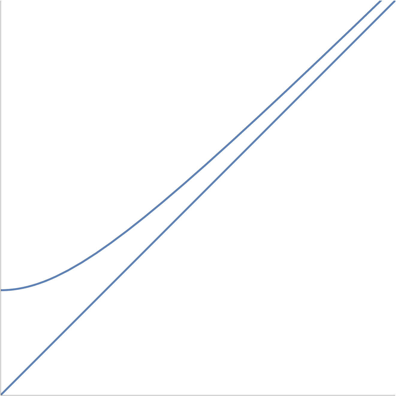
Imagine that we have a windowed source function \( j(y^0, \By) \), as sketched in fig. 5.

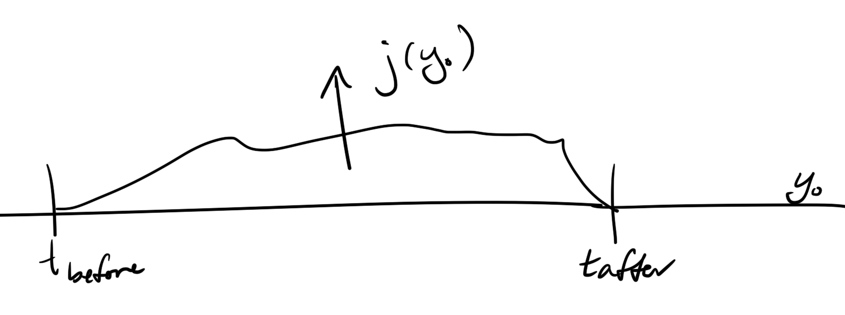
fig. 5. Finite window impulse response.


\begin{equation}\label{eqn:qftLecture12:460}
\evalbar{\phi(x)}{x^0 > t_{\text{after}}}
= \phi_0(x)
+ i \int d^4 y
\lr{
\int \frac{d^3 p}{(2\pi)^3 2 \omega_\Bp } e^{-i p \cdot (x – y)} j(y)

\int \frac{d^3 p}{(2\pi)^3 2 \omega_\Bp } e^{i p \cdot (x – y)} j(y)
}
\end{equation}

define
\begin{equation}\label{eqn:qftLecture12:480}
\tilde{j}(p) = \int d^4 y e^{i p \cdot y} j(y),
\end{equation}
which gives
\begin{equation}\label{eqn:qftLecture12:500}
\evalbar{\phi(x)}{x^0 > t_{\text{after}}}
= \phi_0(x)
+ i \int \frac{d^3 p }{(2 \pi)^3}
\inv{
2 \omega_\Bp }
\evalbar{
\lr{
e^{-i p \cdot x} \tilde{j}(p)
– e^{i p \cdot x} \tilde{j}(-p)
}
}{p_0 = \omega_\Bp}.
\end{equation}
We will interpret this in the next lecture, and start in on Feynman diagrams.

References

New aggregate notes collection for UofT phy2403 Quantum Field Theory I

October 21, 2018 phy2403 , ,

I’ve uploaded a new aggregate notes collection of my UofT phy2403 Quantum Field Theory I class notes (taught by Prof. Erich Poppitz), which now includes up to Wed Oct 17th’s lecture 11 (but doesn’t have my problem set I solution)

  • 1 Introduction
  • 1.1 What is a field?
  • 1.2 Scales.
  • 1.2.1 Bohr radius
  • 1.2.2 Compton wavelength.
  • 1.2.3 Relations.
  • 2 Units, scales, and Lorentz transformations.
  • 2.1 Natural units.
  • 2.2 Gravity.
  • 2.3 Cross section.
  • 2.4 Lorentz transformations.
  • 3 Lorentz transformations and a scalar action.
  • 3.1 Determinant of Lorentz transformations.
  • 3.2 Field theory.
  • 3.3 Actions.
  • 3.4 Problems.
  • 4 Scalar action, least action principle, Euler-Lagrange equations for a field, canonical quantization.
  • 4.1 Principles cont.
  • 4.2 d = 2 .
  • 4.3 d = 3 .
  • 4.4 d = 4 .
  • 4.5 d = 5 .
  • 4.6 Least action principle (classical field theory)
  • 4.7 Canonical quantization.
  • 5 Klein-Gordon equation, SHOs, momentum space representation, raising and lowering operators.
  • 5.1 Canonical quantization.
  • 5.2 Momentum space representation.
  • 6 Canonical quantization, Simple Harmonic Oscillators, Symmetries
  • 6.1 Quantization of Field Theory.
  • 6.2 Free Hamiltonian.
  • 6.3 QM SHO review.
  • 6.4 Discussion.
  • 6.5 Switching gears: Symmetries.
  • 7 Symmetries, translation currents, energy momentum tensor.
  • 7.1 Symmetries.
  • 7.2 Spacetime translation.
  • 8 1st Noether theorem, spacetime translation current, energy momentum tensor, dilatation current.
  • 8.1 1st Noether theorem.
  • 8.2 Unitary operators.
  • 8.3 Continuous symmetries.
  • 8.4 Classical scalar theory.
  • 9 Unbroken and spontaneously broken symmetries, Higgs Lagrangian, scale invariance, Lorentz invariance, angular momentum quantization
  • 9.1 Last time.
  • 9.2 Examples of symmetries.
  • 9.3 Scale invariance.
  • 9.4 Lorentz invariance.
  • 10 Lorentz boosts, generator of spacetime translation, Lorentz invariant field representation.
  • 10.1 Lorentz transform symmetries.
  • 10.2 Transformation of momentum states.
  • 11 Microcausality, Lorentz invariant measure, retarded time SHO Green’s function.
  • 11.1 Relativistic normalization.
  • 11.2 Spacelike surfaces.
  • 11.3 Condition on microcausality.
  • 11.4 Harmonic oscillator.
  • 11.5 Field theory (where we are going).
  • 12 Independent study problems
  • Appendices
  • A Useful formulas and review
  • Index
  • Bibliography

PHY2403H Quantum Field Theory. Lecture 11: Momentum matrix elements, spacelike surfaces, microcausality, Lorentz invariant measure, wave function Green’s function, retarded time contour, advanced time contour. Taught by Prof. Erich Poppitz

October 20, 2018 phy2403 , , , , , ,

[Click here for a PDF of this post with nicer formatting]

DISCLAIMER: Very rough notes from class, with some additional side notes.

These are notes for the UofT course PHY2403H, Quantum Field Theory I, taught by Prof. Erich Poppitz fall 2018.

Relativistic normalization.

We will continue looking at the generator of spacetime translation \( \hatU(\Lambda) \), which has the property
\begin{equation}\label{eqn:qftLecture11:40}
\hatU(\Lambda) \ket{0} = \ket{0},
\end{equation}

That is
\begin{equation}\label{eqn:qftLecture11:760}
\hatU(\Lambda) = \mathbf{1} + \text{operators that anhillate the vacuum state}.
\end{equation}

The action on a field was
\begin{equation}\label{eqn:qftLecture11:60}
\hatU(\Lambda)
\phihat(x) \hatU^\dagger(\Lambda)
= \phihat(\Lambda x),
\end{equation}
and the action on the anhillation operator was
\begin{equation}\label{eqn:qftLecture11:300}
\hatU(\Lambda)
\sqrt{ 2 \omega_\Bp } \hat{a}_\Bp
\hatU^\dagger(\Lambda)
=
\sqrt{ 2 \omega_{\Lambda \Bp} } \hat{a}_{\Lambda \Bp}.
\end{equation}

If \( \ket{\Bp_1} \) is the one particle state with momentum \( \Bp_1 \), then that momentum state can be generated from the ground state with the following normalized creation operation
\begin{equation}\label{eqn:qftLecture11:780}
\ket{\Bp_1} = \sqrt{ 2 \omega_{\Bp_1} } \hat{a}_{\Bp_1}^\dagger \ket{0}.
\end{equation}

We can compute the matrix element between two matrix states using the creation operator representation
\begin{equation}\label{eqn:qftLecture11:80}
\begin{aligned}
\braket{\Bp_2}{\Bp_1}
&=
\sqrt{ 2 \omega_{\Bp_1} }
\sqrt{ 2 \omega_{\Bp_2} }
\bra{0}
\hat{a}_{\Bp_2}
\hat{a}_{\Bp_1}^\dagger
\ket{0} \\
&=
\sqrt{ 2 \omega_{\Bp_1} }
\sqrt{ 2 \omega_{\Bp_2} }
\bra{0}
\lr{
\hat{a}_{\Bp_1}^\dagger
\hat{a}_{\Bp_2}
+
i (2 \pi)^3 \delta^3(\Bp – \Bq)
} \\
&=
\sqrt{ 2 \omega_{\Bp_1} }
\sqrt{ 2 \omega_{\Bp_2} }
(2 \pi)^3 \delta^3(\Bp_1 – \Bp_2) \\
&=
2 \omega_{\Bp_1}
(2 \pi)^3 \delta^3(\Bp_1 – \Bp_2).
\end{aligned}
\end{equation}

Spacelike surfaces.

fig. 0. Constant spacelike surface.

If \( x^\mu, p^\mu \) are four vectors, then \( p^\mu x_\mu = \text{invariant} = {p’}^\mu x’_\mu \). The light cone is the surface \( p_0^2 = \Bp^2 \), whereas timelike four-momentum form a parabaloid surface \( p_0^2 – \Bp^2 = m^2 \) (i.e. \( E = \sqrt{ m^2 c^4 + \Bp^2 c^2 } \)).
The surface for constant spacelike points (i.e. all related by a Lorentz transformation) is illustrated in fig. 0. A boost moves a point up or down that surface along the energy axis. It is therefore possible to use a sequence of boost and rotation to transform a point \( (E, \Bp) \rightarrow (-E, \Bp) \rightarrow (-E, -\Bp) \). That is, any spacelike four-vector \( x \) may be transformed to \( -x \) using a Lorentz transformation.

Condition on microcausality.

We defined operators \( \phihat(\Bx) \), which was a Hermitian operator for the real scalar field. For the complex scalar field we used \( \phihat(\Bx) = (\phihat_1 + \phihat_2)/\sqrt{2} \), where each of \( \phihat_1, \phihat_2 \) were Hermitian operators. i.e. we can think of these operators as “observables”, that is \( \phihat(\Bx) = \phihat^\dagger(\Bx) \).

We now want to show that these operators commute at spacelike separations, and see how this relates to the question of causality. In particular, we want to see that an observation of one operator, will not effect the measurement of the other.

The condition of microcausality is
\begin{equation*}
\antisymmetric{\phihat(x)}{\phihat(y)} = 0
\end{equation*}
if \( x \sim y \), that is \( (x – y)^2 < 0 \). That is, \( x, y \) are spacelike separated.

We wrote

\begin{equation}\label{eqn:qftLecture11:160}
\phihat(x)
=
\int \frac{d^3 p}{(2 \pi)^3 \sqrt{2 \omega_\Bp}}
\evalbar{
e^{-i p \cdot x} }{p^0 = \omega_\Bp} \hat{a}_\Bp
+
\int \frac{d^3 p}{(2 \pi)^3 \sqrt{2 \omega_\Bp}}
\evalbar{
e^{i p \cdot x} }{p^0 = \omega_\Bp} \hat{a}^\dagger_\Bp
,
\end{equation}
or \( \phihat(x) = \phihat_{-}(x) + \phihat_{+}(x) \), where
\begin{equation}\label{eqn:qftLecture11:180}
\begin{aligned}
\phihat_{-}(x) &=
\int \frac{d^3 p}{(2 \pi)^3 \sqrt{2 \omega_\Bp}}
\evalbar{
e^{-i p \cdot x} }{p^0 = \omega_\Bp} \hat{a}_\Bp \\
\phihat_{+}(x) &=
\int \frac{d^3 p}{(2 \pi)^3 \sqrt{2 \omega_\Bp}}
\evalbar{
e^{i p \cdot x} }{p^0 = \omega_\Bp} \hat{a}^\dagger_\Bp
\end{aligned}
\end{equation}

Compute the commutator
\begin{equation}\label{eqn:qftLecture11:200}
\begin{aligned}
D(x)
&= \antisymmetric{\phihat_{-}(x)}{\phihat_{+}(0)} \\
&=
\int \frac{d^3 p}{(2 \pi)^3 \sqrt{2 \omega_\Bp}}
\evalbar{ e^{-i p \cdot x} }{p^0 = \omega_\Bp}
\int \frac{d^3 k}{(2 \pi)^3 \sqrt{2 \omega_\Bk}}
\evalbar{ e^{i k \cdot 0} }{k^0 = \omega_\Bk}
\antisymmetric{\hat{a}_\Bp }{\hat{a}_\Bk^\dagger } \\
&=
\int \frac{d^3 p}{(2 \pi)^3 \sqrt{2 \omega_\Bp}}
\evalbar{ e^{-i p \cdot x} }{p^0 = \omega_\Bp}
\int \frac{d^3 k}{(2 \pi)^3 \sqrt{2 \omega_\Bk}}
(2 \pi)^3 \delta^3(\Bp – \Bk),
\end{aligned}
\end{equation}
\begin{equation}\label{eqn:qftLecture11:800}
\boxed{
D(x)
=
\int \frac{d^3 p}{(2 \pi)^3 2 \omega_\Bp}
\evalbar{ e^{-i p \cdot x} }{p^0 = \omega_\Bp}.
}
\end{equation}

Now about the commutator at two spacetime points
\begin{equation}\label{eqn:qftLecture11:220}
\begin{aligned}
\antisymmetric{\phihat(x)}{\phihat(y)}
&=
\antisymmetric{\phihat_{-}(x) + \phihat_{+}(x)}{\phihat_{-}(y) + \phihat_{+}(y)} \\
&=
\antisymmetric{\phihat_{-}(x)}{\phihat_{+}(y)}
+
\antisymmetric{\phihat_{+}(x)}{\phihat_{-}(y)} \\
&=
-D(y – x) + D(x – y)
\end{aligned}
\end{equation}

Find
\begin{equation}\label{eqn:qftLecture11:240}
\begin{aligned}
\antisymmetric{\phihat(x)}{\phihat(y)} &= D(x – y) – D(y – x) \\
\antisymmetric{\phihat(x)}{\phihat(0)} &= D(x) – D(- x)
\end{aligned}
\end{equation}

Let’s look at \( D(x) \), \ref{eqn:qftLecture11:800}, a bit more closely.

Claim:

D(x) is Lorentz invariant (has the same value for all \( x^\mu, {x’}^\mu \)

We can see this by writing this out as
\begin{equation}\label{eqn:qftLecture11:280}
D(x)
=
\int \frac{d^3 p}{(2 \pi)^3 } dp^0
\delta( p_0^2 – \Bp^2 – m^2) \Theta(p^0)
e^{-i p \cdot x}
\end{equation}

The exponential is Lorentz invariant, and the delta function has been put into a Lorentz invariant form.

Claim 1:

\( D(x) = D(x’) \) where \( x^2 = {x’}^2 \).

Claim 2:

\( x^\mu, -x^\mu \) are related by Lorentz transformations if \( x^2 < 0 \).

From the figure, we see that \( D(x) = D(-x) \) for a spacelike point, which implies that \( \antisymmetric{\phihat(x)}{\phihat(0)} = 0 \) for a spacelike point \( x \).

We’ve shown this for free fields, but later we will see that this is the case for interacting fields too.

Harmonic oscillator.

\begin{equation}\label{eqn:qftLecture11:320}
L = \inv{2} \qdot^2 – \frac{\omega^2}{t} q^2 – j(t) q
\end{equation}

The term \( j(t) \) shifts the origin in a time dependent fashion (graphical illustration in class wiggling a hockey stick, as a sample of a harmonic oscillator).

\begin{equation}\label{eqn:qftLecture11:340}
H = \frac{p^2}{2} + \frac{\omega^2}{t} q^2 + j(t) q
\end{equation}

\begin{equation}\label{eqn:qftLecture11:360}
\begin{aligned}
i \qdot_H(t) &= \antisymmetric{q_H}{H} = i p_H \\
i \pdot_H(t) &= \antisymmetric{p_H}{H} = -i \omega^2 q_H – i j(t)
\end{aligned}
\end{equation}

\begin{equation}\label{eqn:qftLecture11:380}
\ddot{q}_H(t) = – \omega^2 q_H(t) – j(t)
\end{equation}
or
\begin{equation}\label{eqn:qftLecture11:400}
(\partial_{tt} + \omega^2 ) q_H(t) = – j(t)
\end{equation}

\begin{equation}\label{eqn:qftLecture11:420}
q_H(t) = q_H^0( t ) +
\int G_R(t – t’) j(t’) dt’
\end{equation}

This solves the equation provided \( G_R(t – t’) \) has the property that
\begin{equation}\label{eqn:qftLecture11:440}
\boxed{
(\partial_{tt} + \omega^2)
G_R(t – t’)
= – \delta(t – t’)
}
\end{equation}

That is
\begin{equation}\label{eqn:qftLecture11:460}
(\partial_{tt} + \omega^2)
q_H(t) =
(\partial_{tt} + \omega^2)
q_H^0( t )
+
(\partial_{tt} + \omega^2)
\int G_R(t – t’) j(t’) dt’
\end{equation}

This function \( G_R \) is called the retarded Green’s function. We want to find this function, and as usual, we do this by taking the Fourier transform of \ref{eqn:qftLecture11:440}

\begin{equation}\label{eqn:qftLecture11:480}
\begin{aligned}
\int dt e^{i p t}
(\partial_{tt} + \omega^2) G_R(t – t’)
&=
-\int_{-\infty}^\infty dt e^{i p t}
\delta(t – t’) \\
&= – e^{i p t’}
\end{aligned}
\end{equation}

Let
\begin{equation}\label{eqn:qftLecture11:500}
G(t – t’) = \int \frac{dp }{2 \pi} e^{- i p'(t – t’)} \tilde{G}(p’),
\end{equation}
so

\begin{equation}\label{eqn:qftLecture11:520}
\begin{aligned}
– e^{i pt’}
&=
\int dt e^{i p t}
(\partial_{tt} + \omega^2)
\int \frac{dp’}{2 \pi} e^{- i p'(t – t’)} \tilde{G}(p’) \\
&=
\int dt e^{i p t} \int
\frac{dp’}{2 \pi} \lr{ -{p’}^2 + \omega^2 } e^{- i p'(t – t’)} \tilde{G}(p’) \\
&=
\int dp’ \lr{ -{p’}^2 + \omega^2 } e^{i p’ t’} \delta(p – p’) \tilde{G}(p’) \\
&=
\lr{ -{p}^2 + \omega^2 } \tilde{G}(p) e^{i p t’}
\end{aligned}
\end{equation}

so
\begin{equation}\label{eqn:qftLecture11:540}
\tilde{G}(p)
= \inv{p^2 – \omega^2}
\end{equation}

Now

\begin{equation}\label{eqn:qftLecture11:560}
G(t)
= \int \frac{dp}{2 \pi} e^{-i p t}
\tilde{G}(p)
\end{equation}

Let’s write the momentum space Green’s function as
\begin{equation}\label{eqn:qftLecture11:580}
\tilde{G}(p)
= \inv{(p – \omega)(p + \omega)}
\end{equation}

The solution contained
\begin{equation}\label{eqn:qftLecture11:600}
\int G(t – t’) j(t’) dt’.
\end{equation}
Suppose \( j(t) = 0 \) for all \( t < t_0 \). We want the effect of \( j(t) \) to be felt in the future, for example, \(j(t) \) is an impulse starting at some time. We want \( G(t) \) to vanish at negative times.

We want the integral
\begin{equation}\label{eqn:qftLecture11:620}
G(t)
= \int \frac{dp}{2 \pi} e^{-i p t}
\inv{(p – \omega)(p + \omega)}
\end{equation}
to vanish when \( t < 0 \). Start with \( t > 0 \) (that is \( t’ < t \)), so that \( e^{-i p t} = e^{-i p \Abs{t}} \) which means that we have to integrate over a lower plane contour like fig. 1, because the imaginary part of \( p \) is negative, but for \( t < 0 \) (that is \( t’ > t \)), we want an upper plane contour like fig. 2.

fig. 1. Lower plane contour.


fig. 2. Upper plane contour.


Question: since we are integrating over the real line, how can we get away with deforming the contour?
Answer: it works. If we do this we get a Green’s function that makes sense (better answer later?)

We add an infinite circle, so that we can integrate over a closed contour, and pick the contour so that it is zero for \( t < 0 \) and non-zero (enclosed poles) for \( t > 0 \).

\begin{equation}\label{eqn:qftLecture11:640}
\begin{aligned}
G_R(t > 0)
&= \int_C \frac{dp}{2 \pi} e^{-i p t}
\inv{(p – \omega)(p + \omega)} \\
&=
\inv{2 \pi} (-2 \pi i) \lr{
\frac{e^{-i \omega t}}{2 \omega}

\frac{e^{i \omega t}}{2 \omega}
} \\
&=
-\frac{\sin(\omega t)}{\omega}.
\end{aligned}
\end{equation}

Now we write the Green’s function for all time as
\begin{equation}\label{eqn:qftLecture11:660}
\boxed{
G_R(t) =
-\frac{\sin(\omega t)}{\omega} \Theta(t).
}
\end{equation}

The question of what contour to pick can now be justified by the result, since this satisfies fig. 3). In particular, the bumps up and down contour will be used to derive the “Feynman propagator” that we’ll use later.

fig. 3. All possible deformations around the poles.


Field theory (where we are going).

We will consider a massive real scalar field theory with an external source with action

\begin{equation}\label{eqn:qftLecture11:680}
S = \int d^4 x \lr{
\inv{2} \partial_\mu \phi \partial^\mu \phi – \frac{m^2}{2} \phi^2 + j(x) \phi(x)
}
\end{equation}

We don’t have examples of currents that create scalar fields, but to study such as system, recall that
in electromagnetism we added sources to the field by adding a term like
\begin{equation}\label{eqn:qftLecture11:700}
\int d^4 x A^\mu(x) j_\mu(x),
\end{equation}
to our action.

The equation of motion can be found to be
\begin{equation}\label{eqn:qftLecture11:720}
\lr{ \partial_\mu \partial^\mu + m^2 } \phi(x) = j(x).
\end{equation}

We want to study the Green’s function of this Klien-Gordon equation, defined to obey
\begin{equation}\label{eqn:qftLecture11:740}
\lr{ \partial_\mu \partial^\mu + m^2 }_x G(x – y) = -i \delta^4(x – y),
\end{equation}
where the \( -i \) factor is for convienience.
This is analogous to the Green’s function that we just studied for the QM harmonic oscillator.

Question: Compute \( D(x-y) \) from the commutator.

Generalize the derivation \ref{eqn:qftLecture11:800} by computing the commutator at two different space time points \( x, y \).

Answer

Let
\begin{equation}\label{eqn:qftLecture11:860}
\begin{aligned}
D(x – y)
&= \antisymmetric{\phihat_{-}(x)}{\phihat_{+}(y)} \\
&=
\int \frac{d^3 p}{(2 \pi)^3 \sqrt{2 \omega_\Bp}}
\evalbar{ e^{-i p \cdot x} }{p^0 = \omega_\Bp}
\int \frac{d^3 k}{(2 \pi)^3 \sqrt{2 \omega_\Bk}}
\evalbar{ e^{i k \cdot y} }{k^0 = \omega_\Bk}
\antisymmetric{\hat{a}_\Bp }{\hat{a}_\Bk^\dagger } \\
&=
\int \frac{d^3 p}{(2 \pi)^3 \sqrt{2 \omega_\Bp}}
\evalbar{ e^{-i p \cdot x} }{p^0 = \omega_\Bp}
\int \frac{d^3 k}{(2 \pi)^3 \sqrt{2 \omega_\Bk}}
\evalbar{ e^{i k \cdot y} }{k^0 = \omega_\Bk}
(2 \pi)^3 \delta^3(\Bp – \Bk) \\
&=
\int \frac{d^3 p}{(2 \pi)^3 2 \omega_\Bp}
\evalbar{ e^{-i p \cdot (x – y)} }{p^0 = \omega_\Bp}.
\end{aligned}
\end{equation}

Question: Verification of harmonic oscillator Green’s function.

Take the derivatives of a convolution of the Green’s function \ref{eqn:qftLecture11:660} to show that it satisifies \ref{eqn:qftLecture11:440}.

Answer

Let
\begin{equation}\label{eqn:qftLecture11:880}
\begin{aligned}
q(t)
&= \int_{-\infty}^\infty G(t – t’) j(t’) dt’ \\
&= -\inv{\omega} \int_{-\infty}^\infty \sin(\omega(t – t’)) \Theta(t – t’) j(t’) dt’.
\end{aligned}
\end{equation}
We are free to add any \( q_0(t) \) that satisfies the homogeneous wave equation \( q_0”(t) + \omega^2 q_0(t) = 0 \) to our assumed convolution solution \ref{eqn:qftLecture11:880}, but that isn’t interesting for this exersize.
Since \( \Theta(t – t’) = 0 \) for \( t – t’ < 0 \), or \( t’ > t \), the convolution can be written as
\begin{equation}\label{eqn:qftLecture11:900}
q(t)
= -\inv{\omega} \int_{-\infty}^t \sin(\omega(t – t’)) j(t’) dt’,
\end{equation}
which is now in a convient form to take derivatives. We have contributions from the boundary’s time dependence and from the integrand. In particular
\begin{equation}\label{eqn:qftLecture11:920}
\ddt{} \int_{a(t)}^{b(t)} g(x, t) dx
=
g(b(t)) b'(t) – g(a(t)) a'(t) + \int_a^b \frac{\partial}{\partial t} g(x, t) dx.
\end{equation}
Assuming that \( j(-\infty) = 0 \), this gives
\begin{equation}\label{eqn:qftLecture11:940}
\begin{aligned}
\ddt{q(t)}
&=
-\inv{\omega} \evalbar{\sin(\omega(t – t’)) j(t’) }{t’ = t}
-\int_{-\infty}^t \cos(\omega(t – t’)) j(t’) dt’ \\
&=
-\int_{-\infty}^t \cos(\omega(t – t’)) j(t’) dt’.
\end{aligned}
\end{equation}
For the second derivative we have
\begin{equation}\label{eqn:qftLecture11:960}
\begin{aligned}
q”(t)
&=
– \evalbar{ \cos(\omega(t – t’)) j(t’) }{t’ = t}
+\omega \int_{-\infty}^t \sin(\omega(t – t’)) j(t’) dt’ \\
&=
-j(t) -\omega^2
\int_{-\infty}^t \frac{-\sin(\omega(t – t’))}{\omega} j(t’) dt’,
\end{aligned}
\end{equation}
or
\begin{equation}\label{eqn:qftLecture11:980}
q”(t) = -j(t) – \omega^2 q(t),
\end{equation}
which is our forced Harmonic oscillator equation.

PHY2403H Quantum Field Theory. Lecture 10: Lorentz boosts, generator of spacetime translation, Lorentz invariant field representation. Taught by Prof. Erich Poppitz

October 16, 2018 phy2403 , , , , ,

[Click here for a PDF of this post with nicer formatting]

DISCLAIMER: Very rough notes from class, with some additional side notes.

These are notes for the UofT course PHY2403H, Quantum Field Theory I, taught by Prof. Erich Poppitz fall 2018.

Lorentz transform symmetries.

From last time, recall that an infinitesimal Lorentz transform has the form
\begin{equation}\label{eqn:qftLecture10:20}
x^\mu \rightarrow x^\mu + \omega^{\mu\nu} x_\nu,
\end{equation}
where
\begin{equation}\label{eqn:qftLecture10:40}
\omega^{\mu\nu} = -\omega^{\nu\mu}
\end{equation}

We showed last time that \( \omega^{ij} \) induces a rotation, and will show today that \( \omega^{0i} \) is a boost.

We introduced a three index current, factoring out explicit dependence on the incremental Lorentz transform tensor \( \omega^{\mu\nu} \) as follows
\begin{equation}\label{eqn:qftLecture10:80}
J^{\nu \mu\rho} = \inv{2} \lr{ x^\rho T^{\nu\mu} – x^\mu T^{\nu\rho} },
\end{equation}
and can easily show that this current has the desired zero four-divergence property
\begin{equation}\label{eqn:qftLecture10:100}
\begin{aligned}
\partial_\nu J^{\nu \mu\rho}
&= \inv{2} \lr{
(\partial_\nu x^\rho) T^{\nu\mu}
+
x^\rho {\partial_\nu T^{\nu\mu} }
– (\partial_\nu x^\mu) T^{\nu\rho}
– x^\mu {\partial_\nu T^{\nu\rho} }
} \\
&= \inv{2} \lr{
(\partial_\nu x^\rho) T^{\nu\mu}
– (\partial_\nu x^\mu) T^{\nu\rho}
} \\
&= \inv{2} \lr{
T^{\rho\mu}
+
– T^{\mu\rho}
} \\
&= 0,
\end{aligned}
\end{equation}
since the energy-momentum tensor is symmetric.

Defining charge in the usual fashion \( Q = \int d^3 x j^0 \), so we can define a charge for each pair of indexes \( \mu\nu \), and in particular
\begin{equation}\label{eqn:qftLecture10:120}
Q^{0k} = \int d^3 x J^{0 0 k} = \inv{2} \int d^3 x \lr{ x^k T^{00} – x^0 T^{0k} }
\end{equation}
\begin{equation}\label{eqn:qftLecture10:540}
\begin{aligned}
\dot{Q}^{0k}
&= \int d^3 x \dot{J}^{0 0k} \\
&= \inv{2} \int d^3 x \lr{ x^k \dot{T}^{00} – x^0 \dot{T}^{0k} }
\end{aligned}
\end{equation}

However, since \( 0 = \partial_\mu T^{\mu \nu} = \dot{T}^{0 \nu} + \partial_j T^{j \nu} \), or \( \dot{T}^{0 \nu} = -\partial_j T^{j \nu} \),
\begin{equation}\label{eqn:qftLecture10:560}
\begin{aligned}
\dot{Q}^{0k}
&= \inv{2} \int d^3 x \lr{ x^k (-\partial_j T^{j0}) – T^{0k} – x^0 (-\partial_j T^{jk}) } \\
&= \inv{2} \int d^3 x \lr{
\partial_j (-x^k T^{j0}) + (\partial_j x^k) T^{j0}
– T^{0k} + x^0 \partial_j T^{jk}
} \\
&= \inv{2} \int d^3 x \lr{
\partial_j (-x^k T^{j0}) + {T^{k0}}
– {T^{0k}} + x^0 \partial_j T^{jk}
} \\
&= \inv{2} \int d^3 x \lr{
\partial_j (-x^k T^{j0})
+ x^0 \partial_j T^{jk}
} \\
&= \inv{2} \int d^3 x
\partial_j \lr{
-x^k T^{j0}
+ x^0 T^{jk}
},
\end{aligned}
\end{equation}
which leaves just surface terms, so \( \dot{Q}^{0k} = 0 \).

Quantizing:

From our previous identification
\begin{equation}\label{eqn:qftLecture9:560}

{T^\nu}_\mu =
-\partial^\nu \phi \partial_\mu \phi + {\delta^{\nu}}_\mu \LL,
\end{equation}
we have
\begin{equation}\label{eqn:qftLecture10:580}
T^{\nu\mu} = \partial^\nu \phi \partial^\mu \phi – g^{\nu\mu} \LL,
\end{equation}
or
\begin{equation}\label{eqn:qftLecture10:600}
\begin{aligned}
T^{00}
&= \partial^0 \phi \partial^0 \phi – \inv{2} \lr{ \partial_0 \phi \partial^0 \phi + \partial_k \phi \partial^k \phi } \\
&= \inv{2} \partial^0 \phi \partial^0 \phi – \inv{2} (\spacegrad \phi)^2,
\end{aligned}
\end{equation}
and
\begin{equation}\label{eqn:qftLecture10:620}
T^{0k} = \partial^0 \phi \partial^k \phi,
\end{equation}
so we may quantize these energy momentum tensor components as
\begin{equation}\label{eqn:qftLecture10:640}
\begin{aligned}
\hatT^{00} &= \inv{2} \hat{\pi}^2 + \inv{2} (\spacegrad \phihat)^2 \\
\hatT^{0k} &= \inv{2} \hat{\pi} \partial^k \phihat.
\end{aligned}
\end{equation}

We can now start computing the commutators associated with the charge operator. The first of those commutators is
\begin{equation}\label{eqn:qftLecture10:140}
\antisymmetric{\hatT^{00}(\Bx)}{\phihat(\By)}
=
\inv{2}
\antisymmetric{\hat{\pi}^2(\Bx)}{\phihat(\By)},
\end{equation}
which can be evaluated using the field commutator analogue of \( \antisymmetric{F(p)}{q} = i F’ \) which is
\begin{equation}\label{eqn:qftLecture10:660}
\antisymmetric{F(\hat{\pi}(\Bx))}{\phihat(\By)} = -i \frac{dF}{d \hat{\pi}} \delta(\Bx – \By),
\end{equation}
to give
\begin{equation}\label{eqn:qftLecture10:680}
\antisymmetric{\hatT^{00}(\Bx)}{\phihat(\By)}
= -i \delta^3(\Bx – \By) \hat{\pi}(\Bx)
\end{equation}

The other required commutator is
\begin{equation}\label{eqn:qftLecture10:160}
\begin{aligned}
\antisymmetric{\hatT^{0i}(\Bx)}{\phihat(\By)}
&=
\antisymmetric{\hat{\pi}(\Bx)\partial^i \phihat(\Bx)}{\phihat(\By)} \\
&=
\partial^i \phihat(\Bx)
\antisymmetric{\hat{\pi}(\Bx)
}{\phihat(\By)} \\
&= -i \delta^3(\Bx – \By) \partial^i \phihat(\Bx),
\end{aligned}
\end{equation}

The charge commutator with the field can now be computed
\begin{equation}\label{eqn:qftLecture10:180}
\begin{aligned}
i \epsilon \antisymmetric{\hatQ^{0k}}{\phihat(\By)}
&=
i
\frac{\epsilon}{2} \int d^3 x
\lr{
x^k
\antisymmetric{\hatT^{00}}{\phihat(\By)}

x^0
\antisymmetric{\hatT^{0k}}{\phihat(\By)}
} \\
&=
\frac{\epsilon}{2} \lr{ y^k \hat{\pi}(\By) – y^0 \partial^k \phihat(\By) } \\
&=
\frac{\epsilon}{2} \lr{ y^k \dot{\phihat}(\By) – y^0 \partial^k \phihat(\By) },
\end{aligned}
\end{equation}
so to first order in \( \epsilon \)
\begin{equation}\label{eqn:qftLecture10:200}
e^{i \epsilon \hatQ^{0k} } \phihat(\By)
e^{-i \epsilon \hatQ^{0k} }
=
\phihat(\By)
+ \frac{\epsilon}{2} y^k \dot{\phihat}(\By)
+ \frac{\epsilon}{2} y^0 \partial_k \phihat(\By)
\end{equation}

For example, with \( k = 1 \)
\begin{equation}\label{eqn:qftLecture10:700}
\begin{aligned}
e^{i \epsilon \hatQ^{0k} } \phihat(\By)
e^{-i \epsilon \hatQ^{0k} }
&=
\phihat(\By)
+ \frac{\epsilon}{2} \lr{
y^1 \dot{\phihat}(\By)
+
y^0 \PD{y^1}{\phihat}(\By)
} \\
&=
\phihat(y^0 + \frac{\epsilon}{2} y^1,
y^1 + \frac{\epsilon}{2} y^2, y^3).
\end{aligned}
\end{equation}

This is a boost. If we compare explicitly to an infinitesimal Lorentz transformation of the coordinates
\begin{equation}\label{eqn:qftLecture10:220}
\begin{aligned}
x^0 \rightarrow x^0 + \omega^{01} x_1 &= x^0 – \omega^{01} x^1 \\
x^1 \rightarrow x^1 + \omega^{10} x_0 &= x^1 – \omega^{01} x_0 = x^1 – \omega^{01} x^0
\end{aligned}
\end{equation}
we can make the identification
\begin{equation}\label{eqn:qftLecture10:240}
\frac{\epsilon}{2} = – \omega^{01}.
\end{equation}

We now have the explicit form of the generator of a spacetime translation

\begin{equation}\label{eqn:qftLecture10:260}
\boxed{
\hatU(\Lambda) = \exp\lr{-i \omega^{0k} \int d^3 x \lr{ \hatT^{00} x^k – \hatT^{0k} x^0 }}
}
\end{equation}

An explicit boost along the x-axis has the form
\begin{equation}\label{eqn:qftLecture10:300}
\hatU(\Lambda) \phihat(t, \Bx)
\hatU^\dagger(\Lambda)
=
\phihat\lr{ \frac{t – vx}{\sqrt{1 – v^2}}, \frac{x – vt}{\sqrt{1 – v^2}}, y, z },
\end{equation}
and more generally
\begin{equation}\label{eqn:qftLecture10:320}
\hatU(\Lambda) \phihat(x) \hatU^\dagger(\Lambda) =
\phihat(\Lambda x)
\end{equation}
where \( x \) is a four vector, \( (\Lambda x)^\mu = {{\Lambda}^\mu}_\nu x^\nu \), and \(
{{\Lambda}^\mu}_\nu
\approx
{{\delta}^\mu}_\nu
+
{{\omega}^\mu}_\nu \).

Transformation of momentum states

In the momentum space representation

\begin{equation}\label{eqn:qftLecture10:340}
\begin{aligned}
\phihat(x)
&=
\int \frac{d^3 p}{(2 \pi)^3 \sqrt{2 \omega_\Bp}} \lr{
e^{i (\omega_\Bp t – \Bp \cdot \Bx)} \hat{a}_\Bp
+
e^{-i (\omega_\Bp t – \Bp \cdot \Bx)} \hat{a}^\dagger_\Bp
} \\
&=
\int \frac{d^3 p}{(2 \pi)^3 \sqrt{2 \omega_\Bp}} \evalbar{
\lr{
e^{i p^\mu x^\mu } \hat{a}_\Bp
+
e^{-i p^\mu x^\mu } \hat{a}^\dagger_\Bp
}
}{p_0 = \omega_\Bp}
\end{aligned}
\end{equation}
\begin{equation}\label{eqn:qftLecture10:720}
\begin{aligned}
\hatU(\Lambda) \phihat(x) \hatU^\dagger(\Lambda)
&=
\phihat(\Lambda x) \\
&=
\int \frac{d^3 p}{(2 \pi)^3 \sqrt{2 \omega_\Bp}} \evalbar{
\lr{
e^{i p^\mu {{\Lambda}^\mu}_\nu x^\nu }
\hat{a}_\Bp
+
e^{-i p^\mu {{\Lambda}^\mu}_\nu x^\nu } \hat{a}^\dagger_\Bp
}
}{p_0 = \omega_\Bp}
\end{aligned}
\end{equation}
This can be put into an explicitly Lorentz invariant form
\begin{equation}\label{eqn:qftLecture10:n}
\begin{aligned}
\phihat(\Lambda x)
&=
\int \frac{dp^0 d^3 p}{(2\pi)^3} \delta(p_0^2 – \Bp^2 – m^2) \Theta(p^0) \sqrt{2 \omega_\Bp}
e^{i p^\mu {{\Lambda}^\mu}_\nu x^\nu }
\hat{a}_\Bp + \text{h.c.} \\
&=
\int \frac{dp^0 d^3 p}{(2\pi)^3}
\lr{
\frac{\delta(p_0 – \omega_\Bp)}{2 \omega_\Bp}
+
\frac{\delta(p_0 + \omega_\Bp)}{2 \omega_\Bp}
}
\Theta(p^0) \sqrt{2 \omega_\Bp} \hat{a}_\Bp + \text{h.c.},
\end{aligned}
\end{equation}
which recovers \ref{eqn:qftLecture10:720} by making use of the delta function identity \( \delta(f(x)) = \sum_{f(x_\conj) = 0} \frac{\delta(x – x_\conj)}{f'(x_\conj)} \), since the \( \Theta(p^0) \) kills the second delta function.

We now have a more explicit Lorentz invariant structure
\begin{equation}\label{eqn:qftLecture10:380}
\phihat(\Lambda x)
=
\int \frac{dp^0 d^3 p}{(2\pi)^3} \delta(p_0^2 – \Bp^2 – m^2) \Theta(p^0) \sqrt{2 \omega_\Bp}
e^{i p^\mu {{\Lambda}^\mu}_\nu x^\nu }
\hat{a}_\Bp + \text{h.c.}
\end{equation}

Recall that a boost moves a spacetime point along a parabola, such as that of fig. 1, whereas a rotation moves along a constant “circular” trajectory of a hyper-paraboloid. In general, a Lorentz transformation may move a spacetime point along any path on a hyper-paraboloid such as the one depicted (in two spatial dimensions) in fig. 2. This paraboloid depict the surfaces of constant energy-momentum \( p^0 = \sqrt{ \Bp^2 + m^2 } \). Because a Lorentz transformation only shift points along that energy-momentum surface, but cannot change the sign of the energy coordinate \( p^0 \), this means that \( \Theta(p^0) \) is also a Lorentz invariant.

fig. 1. One dimensional spacetime surface for constant (p^0)^2 – p^2 = m^2.


fig. 2. Surface of constant squared four-momentum.


Let’s change variables
\begin{equation}\label{eqn:qftLecture10:400}
p^\lambda = {{\Lambda}^\lambda}_\rho {p’}^{\rho}
\end{equation}
so that
\begin{equation}\label{eqn:qftLecture10:420}
\begin{aligned}
p_\mu
{{\Lambda}^\mu}_\nu x^\nu
&=
{{\Lambda}^\lambda}_\rho {p’}^\rho g_{\lambda\nu} {{\Lambda}^\nu}_\sigma x^{\sigma} \\
&=
{p’}^\rho
\lr{ {{\Lambda}^\lambda}_\rho
g_{\lambda\nu} {{\Lambda}^\nu}_\sigma } x^{\sigma} \\
&=
{p’}^\rho g_{\rho\sigma} x^\sigma
\end{aligned}
\end{equation}
which gives
\begin{equation}\label{eqn:qftLecture10:440}
\begin{aligned}
\phihat(\Lambda x)
&=
\int \frac{d{p’}^0 d^3 p’}{(2\pi)^3} \delta({p’}_0^2 – {\Bp’}^2 – m^2) \Theta(p^0) \sqrt{2 \omega_{\Lambda \Bp’}} e^{i p’ \cdot x} \hat{a}_{\Lambda \Bp’} + \text{h.c.} \\
&=
\int \frac{dp^0 d^3 p}{(2\pi)^3} \delta({p}_0^2 – {\Bp}^2 – m^2) \Theta(p^0) \sqrt{2 \omega_{\Lambda \Bp}} e^{i p \cdot x} \hat{a}_{\Lambda \Bp} + \text{h.c.}
\end{aligned}
\end{equation}
Since
\begin{equation}\label{eqn:qftLecture10:460}
\phihat(x)
=
\int \frac{dp^0 d^3 p}{(2\pi)^3} \delta({p}_0^2 – {\Bp}^2 – m^2) \Theta(p^0) \sqrt{2 \omega_{\Bp}} e^{i p \cdot x} \hat{a}_{\Bp} + \text{h.c.}
\end{equation}
we can now conclude that the creation and annihilation operators transform as

\begin{equation}\label{eqn:qftLecture10:480}
\boxed{
\sqrt{2 \omega_{\Lambda \Bp}} \hat{a}_{\Lambda \Bp}
=
\hatU(\Lambda)
\sqrt{2 \omega_{ \Bp}} \hat{a}_{ \Bp}
\hatU^\dagger(\Lambda)
}
\end{equation}

In particular
\begin{equation}\label{eqn:qftLecture10:500}
\sqrt{2 \omega_{ \Bp}} \hat{a}^\dagger_{ \Bp} \ket{0} = \ket{\Bp}
\end{equation}
and noting that \( \hatU(\Lambda) \ket{0} = \ket{0} \) (i.e. the ground state is Lorentz invariant), we have
\begin{equation}\label{eqn:qftLecture10:520}
\begin{aligned}
\sqrt{2 \omega_{\Lambda \Bp}} \hat{a}^\dagger_{\Lambda \Bp} \ket{0}
&=
\hatU(\Lambda) \sqrt{ 2\omega_\Bp} \hat{a}^\dagger_\Bp \hatU^\dagger(\Lambda) \hatU(\Lambda) \ket{0} \\
&=
\hatU(\Lambda) \sqrt{ 2\omega_\Bp} \hat{a}^\dagger_\Bp \ket{0} \\
&=
\hatU(\Lambda) \ket{\Bp}.
\end{aligned}
\end{equation}

PHY2403H Quantum Field Theory. Lecture 8: 1st Noether theorem, spacetime translation current, energy momentum tensor, dilatation current. Taught by Prof. Erich Poppitz

October 14, 2018 phy2403 , , , , , , , , , , , , , ,

[Click here for a PDF of this post with nicer formatting]

DISCLAIMER: Very rough notes from class, with some additional side notes.

These are notes for the UofT course PHY2403H, Quantum Field Theory I, taught by Prof. Erich Poppitz fall 2018.

1st Noether theorem.

Recall that, given a transformation
\begin{equation}\label{eqn:qftLecture8:20}
\phi(x) \rightarrow \phi(x) + \delta \phi(x),
\end{equation}
such that the transformation of the Lagrangian is only changed by a total derivative
\begin{equation}\label{eqn:qftLecture8:40}
\LL(\phi, \partial_\mu \phi) \rightarrow
\LL(\phi, \partial_\mu \phi)
+ \partial_\mu J_\epsilon^\mu,
\end{equation}
then there is a conserved current
\begin{equation}\label{eqn:qftLecture8:60}
j^\mu = \PD{(\partial_\mu \phi)}{\LL} \delta_\epsilon \phi – J_\epsilon^\mu.
\end{equation}
Here \( \epsilon \) is an x-independent quantity (i.e. a \underline{global symmetry}).
This is in contrast to “gauge symmetries”, which can be more accurately be categorized as a redundancy in the description.

As an example, for \( \LL = (\partial_\mu \phi \partial^\mu \phi – m^2 \phi^2)/2 \), let
\begin{equation}\label{eqn:qftLecture8:80}
\phi(x) \rightarrow \phi(x) – a^\mu \partial_\mu \phi
\end{equation}
\begin{equation}\label{eqn:qftLecture8:100}
\LL(\phi, \partial_\mu \phi) \rightarrow
\LL(\phi, \partial_\mu \phi)
– a^\mu \partial_\mu \LL
=
\LL(\phi, \partial_\mu \phi)
+ \partial_\mu \lr{ -{\delta^\mu}_\nu a^\nu \LL }
\end{equation}
Here \( J^\mu_\epsilon = \evalbar{J^\mu_\epsilon}{\epsilon = a^\nu} \), and the current is
\begin{equation}\label{eqn:qftLecture8:120}
J^\mu = (\partial^\mu \phi)(-a^\nu \partial_\nu \phi) + {\delta^{\mu}}_\nu a^\nu \LL.
\end{equation}
In particular, we have one such current for each \( \nu \), and we write
\begin{equation}\label{eqn:qftLecture8:140}
{T^\mu}_\nu =
-(\partial^\mu \phi)(\partial_\nu \phi) + {\delta^{\mu}}_\nu \LL.
\end{equation}
By Noether’s theorem, we must have
\begin{equation}\label{eqn:qftLecture8:160}
\partial_\mu
{T^\mu}_\nu = 0, \quad \forall \nu.
\end{equation}

Check:

\begin{equation}\label{eqn:qftLecture8:1380}
\begin{aligned}
\partial_\mu {T^\mu}_\nu
&=
-(\partial_\mu \partial^\mu \phi)(\partial_\nu \phi)
-(\partial^\mu \phi)(\partial_\mu \partial_\nu \phi)
+ {\delta^{\mu}}_\nu
\partial_\mu \lr{
\inv{2} \partial_\alpha \phi \partial^\alpha \phi – \frac{m^2}{2} \phi^2
} \\
&=
-(\partial_\mu \partial^\mu \phi)(\partial_\nu \phi)
-(\partial^\mu \phi)(\partial_\mu \partial_\nu \phi)
+
\inv{2} (\partial_\nu \partial_\mu \phi) (\partial^\mu \phi )
+
\inv{2} (\partial_\mu \phi) (\partial_\nu \partial^\mu \phi )
– m^2 (\partial_\nu \phi) \phi \\
&=
-\lr{ \partial_\mu \partial^\mu \phi + m^2 \phi }(\partial_\nu \phi)
-(\partial_\mu \phi)(\partial^\mu \partial_\nu \phi)
+
\inv{2} (\partial_\nu \partial^\mu \phi) (\partial_\mu \phi )
+
\inv{2} (\partial_\mu \phi) (\partial_\nu \partial^\mu \phi )
&= 0.
\end{aligned}
\end{equation}

Example: our potential Lagrangian

\begin{equation}\label{eqn:qftLecture8:180}
\LL = \inv{2} \partial^\mu \phi \partial_\nu \phi – \frac{m^2}{2} \phi^2 – \frac{\lambda}{4} \phi^4
\end{equation}
Written with upper indexes
\begin{equation}\label{eqn:qftLecture8:200}
\begin{aligned}
T^{\mu\nu}
&= -(\partial^\mu \phi)(\partial^\nu \phi) + g^{\mu\nu} \LL \\
&= -(\partial^\mu \phi)(\partial^\nu \phi) + g^{\mu\nu} \lr{
\inv{2} \partial^\alpha \phi \partial_\alpha \phi – \frac{m^2}{2} \phi^2 – \frac{\lambda}{4} \phi^4
}
\end{aligned}
\end{equation}

There are 4 conserved currents \( J^{\mu(\nu)} = T^{\mu\nu} \). Observe that this is symmetric (\( T^{\mu\nu} = T^{\nu\mu} \)).

We have four associated charges
\begin{equation}\label{eqn:qftLecture8:220}
Q^\nu = \int d^3 x T^{0 \nu}.
\end{equation}
We call
\begin{equation}\label{eqn:qftLecture8:240}
Q^0 = \int d^3 x T^{0 0},
\end{equation}
the energy density, and call
\begin{equation}\label{eqn:qftLecture8:260}
P^i = \int d^3 x T^{0 i},
\end{equation}
(i = 1,2,3) the momentum density.

writing this out explicitly the energy density is
\begin{equation}\label{eqn:qftLecture8:280}
\begin{aligned}
T^{00}
&= – \dot{\phi}^2 + \inv{2} \lr{ \dot{\phi}^2 – (\spacegrad \phi)^2 – \frac{m^2}{2}\phi^2 – \frac{\lambda}{4} \phi^4} \\
&= -\lr{
\inv{2} \dot{\phi}^2 + \inv{2} (\spacegrad \phi)^2 + \frac{m^2}{2}\phi^2 + \frac{\lambda}{4} \phi^4
},
\end{aligned}
\end{equation}
and
\begin{equation}\label{eqn:qftLecture8:300}
T^{0i} = \partial^0 \phi \partial^i \phi,
\end{equation}
\begin{equation}\label{eqn:qftLecture8:320}
P^{i} = -\int d^3 x\partial^0 \phi \partial^i \phi
\end{equation}
Since the energy density is negative definite (due to an arbitrary choice of translation sign), let’s redefine \( T^{\mu\nu} \) to have a positive sign
\begin{equation}\label{eqn:qftLecture8:340}
T^{00}
\equiv
\inv{2} \dot{\phi}^2 + \inv{2} (\spacegrad \phi)^2 + \frac{m^2}{2} \phi^2 + \frac{\lambda}{4} \phi^4,
\end{equation}
and
\begin{equation}\label{eqn:qftLecture8:360}
P^{i} = \int d^3 x\partial^0 \phi \partial^i \phi
\end{equation}

As an operator we have
\begin{equation}\label{eqn:qftLecture8:380}
\hatQ = \int d^3 x \hatT^{00} =
\int d^3 x
\lr{
\inv{2} \hat{\pi}^2 + \inv{2} (\spacegrad \phihat)^2 + \frac{m^2}{2} \phihat^2 + \frac{\lambda}{4} \phihat^4
}.
\end{equation}
\begin{equation}\label{eqn:qftLecture8:400}
\hatP^{i} = \int d^3 x \hat{\pi} \partial^i \phi
\end{equation}

We showed that
\begin{equation}\label{eqn:qftLecture8:420}
\ddt{\hatO} = i \antisymmetric{\hatH}{\hatO}
\end{equation}
This implied that \( \phihat, \hat{\pi} \) obey the classical EOMs
\begin{equation}\label{eqn:qftLecture8:440}
\ddt{\phihat} = i \antisymmetric{\hat{H}}{\phihat} = \ddt{\hat{\pi}}
\end{equation}
\begin{equation}\label{eqn:qftLecture8:460}
\ddt{\hat{\pi}} = i \antisymmetric{\hatH}{\hat{\pi}} = …
\end{equation}

In terms of creation and annihilation operators (for the \( \lambda = 0 \) free field), up to a constant
\begin{equation}\label{eqn:qftLecture8:480}
\begin{aligned}
\hatH
&= \int d^3 x \hatT^{00} \\
&= \int \frac{d^3 p}{(2 \pi)^3} \omega_\Bp \hat{a}_\Bp^\dagger \hat{a}_\Bp
\end{aligned}
\end{equation}
Can show that:

\begin{equation}\label{eqn:qftLecture8:500}
\begin{aligned}
\hatP^i
&= \int d^3 x \hat{\pi} \partial^i \phihat \\
&= \cdots \\
&= \int \frac{d^3 p}{(2 \pi)^3} p^i \hat{a}_\Bp^\dagger \hat{a}_\Bp
\end{aligned}
\end{equation}
Now we see the energy and momentum as conserved quantities associated with spacetime translation.

Unitary operators

In QM we say that \( \hat{\Bp} \) “generates translations”.

With \( \hat{\Bp} \equiv -i \Hbar \spacegrad \) that translation is
\begin{equation}\label{eqn:qftLecture8:520}
\hatU = e^{i \Ba \cdot \hat{\Bp}} = e^{\Ba \cdot \spacegrad}
\end{equation}

In particular
\begin{equation}\label{eqn:qftLecture8:540}
\bra{\Bx} \hatU \ket{\psi} = e^{\Ba \cdot \hat{\Bp} } \psi(\Bx) = \psi(\Bx + \Ba).
\end{equation}

In one dimension
\begin{equation}\label{eqn:qftLecture8:560}
\begin{aligned}
\hatU \hat{x} \hatU^\dagger
&=
e^{\Ba \cdot \hat{p} } \psi(\Bx)
e^{-\Ba \cdot \hat{p} } \\
&= \hat{\Bx} + a \hat{\mathbf{1}}.
\end{aligned}
\end{equation}
This uses the Baker-Campbell-Hausdorff formula.

Theorem: Baker-Campbell-Hausdorff

\begin{equation}\label{eqn:qftLecture8:600}
e^{B} A e^{-B} = \sum_{n = 0}^\infty \inv{n!} \antisymmetric{B \cdots}{\antisymmetric{B}{A}},
\end{equation}
where the n-th commutator is denoted above

  • \( n = 1 \) : \( \antisymmetric{B}{A} \)
  • \( n = 2 \) : \( \antisymmetric{B}{\antisymmetric{B}{A}} \)
  • \( n = 3 \) : \( \antisymmetric{B}{\antisymmetric{B}{\antisymmetric{B}{A}}} \)

Proof:

\begin{equation}\label{eqn:qftLecture8:620}
\begin{aligned}
f(t)
&= e^{tB} A e^{-tB} \\
&= f(0) + t f'(0) + \frac{t^2}{2} f”(0) + \cdots \frac{t^n}{n!} f^{(n)}(0)
\end{aligned}
\end{equation}

\begin{equation}\label{eqn:qftLecture8:640}
f(0) = A
\end{equation}
\begin{equation}\label{eqn:qftLecture8:660}
\begin{aligned}
f'(t)
&=
e^{tB} B A e^{-tB}
+
e^{tB} A (-B) e^{-tB} \\
&=
e^{tB} \antisymmetric{B}{A} e^{-tB}
\end{aligned}
\end{equation}
\begin{equation}\label{eqn:qftLecture8:680}
\begin{aligned}
f”(t)
&=
e^{tB} B \antisymmetric{B}{A} e^{-tB}
+
e^{tB} \antisymmetric{B}{A} (-B) e^{-tB} \\
&=
e^{tB} \antisymmetric{B}{\antisymmetric{B}{A}} e^{-tB}.
\end{aligned}
\end{equation}
From
\begin{equation}\label{eqn:qftLecture8:700}
f(1)
= f(0) + f'(0) + \inv{2} f”(0) + \cdots \inv{n!} f^{(n)}(0)
\end{equation}
we have
\begin{equation}\label{eqn:qftLecture8:720}
e^{B} A e^{-B} = A +
\antisymmetric{B}{A} + \inv{2} \antisymmetric{B}{\antisymmetric{B}{A}} + \cdots
\end{equation}

Example:
\begin{equation}\label{eqn:qftLecture8:740}
\begin{aligned}
e^{a \partial_x} x e^{-a \partial_x }
&= x + a \antisymmetric{\partial_x}{x} + \cdots \\
&= x + a.
\end{aligned}
\end{equation}

Application:

\begin{equation}\label{eqn:qftLecture8:760}
e^{i \text{Hermitian} } = \text{unitary}
\end{equation}
\begin{equation}\label{eqn:qftLecture8:860}
e^{i \text{Hermitian} } \times
e^{-i \text{Hermitian} }
= 1
\end{equation}
So
\begin{equation}\label{eqn:qftLecture8:780}
\hatU(\Ba) =
e^{i a^j \hat{p}^j }
\end{equation}
is a unitary operator representing finite translations in a Hilbert space.

\begin{equation}\label{eqn:qftLecture8:800}
\begin{aligned}
\hatU(\Ba) \phihat(\Bx) \hatU^\dagger(\Ba)
&=
e^{i a^j \hat{p}^j }
\phihat(\Bx)
e^{-i a^k \hat{p}^k } \\
&=
\phihat(\Bx)
+ i a^j \antisymmetric{\hatP^j}{\phihat(\Bx)} + \frac{-a^{j_1} a^{j_2}}{2} \antisymmetric{\hatP^{j_1}}{\antisymmetric{\hatP^{j_2}}{\phihat(\Bx)}}
\end{aligned}
\end{equation}

\begin{equation}\label{eqn:qftLecture8:820}
\begin{aligned}
\antisymmetric{\hatP^j}{\phihat(\Bx)}
&=
\int d^3 y \antisymmetric{\hat{\pi}(\By) \partial^j \phihat(\By)}{\phihat(\Bx)} \\
&=
\int d^3 y \antisymmetric{\hat{\pi}(\By)}{\phihat(\Bx} \partial^j \phihat(\By) \\
&=
\int d^3 y (-i ) \delta^3(\By – \Bx) \partial^j \phihat(\By) \\
&=
-i \partial^j \phihat(\Bx).
\end{aligned}
\end{equation}

\begin{equation}\label{eqn:qftLecture8:840}
\begin{aligned}
\hatU(\Ba) \phihat(\Bx) \hatU^\dagger(\Ba)
&= \phihat(\Bx) + i a^j (-i) \partial^j \phihat(\Bx) + \cdots \\
&= \phihat(\Bx) + a^j \partial^j \phihat(\Bx) + \cdots \\
&= \phihat(\Bx + \Ba)
\end{aligned}
\end{equation}

Continuous symmetries

For all infinitesimal transformations, continuous symmetries lead to conserved charges \( Q \). In QFT we map these charges to Hermitian operators \( Q \rightarrow \hatQ \). We say that these charges are “generators of the corresponding symmetry” through unitary operators
\begin{equation}\label{eqn:qftLecture8:880}
\hatU = e^{i \text{parameter} \hatQ}.
\end{equation}
These represent the action of the symmetry in the Hilbert space.

Example: spatial translation

\begin{equation}\label{eqn:qftLecture8:900}
\hatU(\Ba) = e^{i \Ba \cdot \hat{\BP}}
\end{equation}

Example: time translation

\begin{equation}\label{eqn:qftLecture8:920}
\hatU(t) = e^{i t \hat{H}}.
\end{equation}

Classical scalar theory

For \( d > 2 \) let’s look at
\begin{equation}\label{eqn:qftLecture8:940}
S =
\int d^d x \lr{
\inv{2} \partial^\mu \phi \partial_\mu \phi – \frac{m^2}{2} \phi^2 – \lambda \phi^{d-2}
}
\end{equation}

Take \( m^2, \lambda \rightarrow 0 \), the free massless scalar field.

We have a shift symmetry in this case since \( \phi(x) \rightarrow \phi(x) + \text{constant} \).
The current is just
\begin{equation}\label{eqn:qftLecture8:960}
\begin{aligned}
j^\mu
&= \PD{(\partial_\mu \phi)}{\phi} \delta \phi – J^\mu \\
&= \PD{(\partial_\mu \phi)}{\phi} \delta \phi \\
&= \text{constant} \times \partial^\mu \phi \\
&= \partial^\mu \phi,
\end{aligned}
\end{equation}
where the constant factor has been set to one.
This current is clearly conserved since \( \partial_\mu J^\mu = \partial_\mu \partial^\mu \phi = 0\) (the equation of motion).

These are called “Goldstein Bosons”.

With \( m = \lambda = 0, d = 4 \) we have

NOTE: We did this in class differently with \( d \ne 4, m, \lambda \ne 0\), and then switched to \( m = \lambda = 0, d = 4\), which was confusing. I’ve reworked my notes to \( d = 4 \) like the supplemental handout that did the same.

\begin{equation}\label{eqn:qftLecture8:980}
S =
\int d^4 x \lr{
\inv{2} \partial^\mu \phi \partial_\mu \phi
}
\end{equation}
Here we have a scale or dilatation invariance
\begin{equation}\label{eqn:qftLecture8:1000}
x \rightarrow x’ = e^{\lambda} x,
\end{equation}
\begin{equation}\label{eqn:qftLecture8:1020}
\phi(x) \rightarrow \phi'(x’) = e^{-\lambda} \phi,
\end{equation}
\begin{equation}\label{eqn:qftLecture8:1040}
d^4 x \rightarrow d^4 x’ = e^{4\lambda} d^4 x,
\end{equation}

The partials transform as
\begin{equation}\label{eqn:qftLecture8:1400}
\partial^\mu \rightarrow
\PD{x’_\mu}{}
=
\PD{x’_\mu}{x_\mu}
\PD{x_\mu}{}
=
e^{-\lambda}
\PD{x_\mu}{}
\end{equation}

so the partial of the field transforms as
\begin{equation}\label{eqn:qftLecture8:1420}
\partial^\mu \phi(x) \rightarrow \PD{x’_\mu}{\phi'(x’)} = e^{-2\lambda} \partial^\mu \phi(x),
\end{equation}
and finally
\begin{equation}\label{eqn:qftLecture8:1060}
(\partial_\mu \phi)^2 \rightarrow e^{-4\lambda} \lr{ \partial_\mu \phi(x) }^2.
\end{equation}

With a \( -4 \lambda \) power in the transformed quadratic term, and \( 4 \lambda \) in the volume element, we see that the action is invariant.

To find Noether current, we need to vary the field and it’s derivatives
\begin{equation}\label{eqn:qftLecture8:1100}
\begin{aligned}
\delta_\lambda \phi
&= \phi'(x) – \phi(x) \\
&= \phi'(e^{-\lambda} x’) – \phi(x) \\
&\approx \phi'(x’ -\lambda x’) – \phi(x) \\
&\approx \phi'(x’) – \lambda {x’}^\alpha \partial_\alpha \phi'(x’) – \phi(x) \\
&\approx (1 – \lambda) \phi(x) – \lambda {x’}^\alpha \partial_\alpha \phi'(x’) – \phi(x) \\
&= – \lambda(1 + x^\alpha \partial_\alpha ) \phi,
\end{aligned}
\end{equation}
where the last step assumes that \( x’ \rightarrow x, \phi’ \rightarrow \phi \), effectively weeding out any terms that are quadratic or higher in \( \lambda \).

Now we need the variation of the derivatives of \( \phi \)
\begin{equation}\label{eqn:qftLecture8:1440}
\delta \partial_\mu \phi(x)
=
\partial_\mu’ \phi'(x) – \partial_\mu \phi(x),
\end{equation}
By \ref{eqn:qftLecture8:1420}
\begin{equation}\label{eqn:qftLecture8:1460}
\begin{aligned}
\partial_\mu’ \phi'(x’)
&=
e^{-2\lambda} \partial_\mu \phi(x) \\
&=
e^{-2\lambda} \partial_\mu \phi(e^{-\lambda} x’) \\
&\approx
e^{-2\lambda} \partial_\mu
\lr{
\phi(x’) – \lambda {x’}^\alpha \partial_\alpha \phi(x’)
} \\
&\approx
\lr{
1 – 2 \lambda
}
\partial_\mu
\lr{
\phi(x’) – \lambda {x’}^\alpha \partial_\alpha \phi(x’)
},
\end{aligned}
\end{equation}
so
\begin{equation}\label{eqn:qftLecture8:1480}
\begin{aligned}
\delta \partial_\mu \phi
&=
– \lambda {x}^\alpha \partial_\alpha \partial_\mu \phi(x)
– 2 \lambda \partial_\mu \phi(x) + O(\lambda^2) \\
&=
– \lambda \lr{
{x}^\alpha \partial_\alpha + 2
}
\partial_\mu \phi(x).
\end{aligned}
\end{equation}

\begin{equation}\label{eqn:qftLecture8:1200}
\begin{aligned}
\delta \LL
&=
(\partial^\mu \phi) \delta (\partial_\mu \phi) \\
&= – \lambda \lr{ 2
\partial_\mu \phi
+ x^\alpha \partial_\alpha
\partial_\mu \phi
}
\partial^\mu \phi,
\end{aligned}
\end{equation}
or
\begin{equation}\label{eqn:qftLecture8:1500}
\begin{aligned}
\frac{\delta \LL }{-\lambda}
&=
4 \LL + x^\alpha \lr{ \partial_\alpha \partial_\mu \phi } \partial^\mu \phi \\
&=
4 \LL + x^\alpha \partial_\alpha \lr{ \LL } \\
&=
{4 \LL} + \partial_\alpha \lr{ x^\alpha \LL } – {\LL \partial_\alpha x^\alpha} \\
&=
\partial_\alpha \lr{ x^\alpha \LL }.
\end{aligned}
\end{equation}
The variation in the Lagrangian density is thus
\begin{equation}\label{eqn:qftLecture8:1520}
\delta \LL = \partial_\mu J^\mu_\lambda = \partial_\mu \lr{ -\lambda x^\mu \LL },
\end{equation}
and the current is
\begin{equation}\label{eqn:qftLecture8:1540}
J^\mu_\lambda = -\lambda x^\mu \LL.
\end{equation}

The Noether current is
\begin{equation}\label{eqn:qftLecture8:1240}
\begin{aligned}
j^\mu
&= \PD{(\partial_\mu \phi)}{\LL} \delta \phi – J^\mu \\
&= -\partial^\mu \phi \lr{ 1 + x^\nu \partial_\nu } \phi + \inv{2} x^\mu \partial_\nu \phi \partial^\nu \phi,
\end{aligned}
\end{equation}
or after flipping signs
\begin{equation}\label{eqn:qftLecture8:1280}
\begin{aligned}
j^\mu_{\text{dil}}
&= \partial^\mu \phi \lr{ 1 + x^\nu \partial_\nu } \phi – \inv{2} x^\mu
\partial_\nu \phi \partial^\nu \phi \\
&= x_\nu \lr{ \partial^\mu \phi \partial^\nu \phi – \inv{2} {\delta^{\nu}}_\mu \partial_\lambda \phi \partial^\lambda \phi }
+ \inv{2} \partial^\mu (\phi^2),
\end{aligned}
\end{equation}

\begin{equation}\label{eqn:qftLecture8:1300}
j^\mu_{\text{dil}} = -x_\nu T^{\nu \mu} + \inv{2} \partial^\mu (\phi^2),
\end{equation}

The current and \( T^{\mu\nu} \) can both be redefined \( j^{\mu’} = j^\mu + \partial_\nu C^{\nu\mu} \) adding an antisymmetric \( C^{\mu\nu} = -C^{\nu\mu} \)

\begin{equation}\label{eqn:qftLecture8:1320}
j^\mu_{\text{dil conformal}} = – x_\nu T^{\nu\mu}_{\text{conformal}}
\end{equation}

\begin{equation}\label{eqn:qftLecture8:1340}
\partial_\mu
j^\mu_{\text{dil conformal}} = – {{T_{\text{conformal}}}^\mu}_\mu
\end{equation}

consequence: \( 0 = T^{00} – T^{11} – T^{22} – T^{33} \), which is essentially
\begin{equation}\label{eqn:qftLecture8:1360}
0 = \rho – 3 p = 0.
\end{equation}