Month: November 2018

New aggregate collection of class notes for phy2403: up to lecture 17.

November 14, 2018 phy2403

I’ve now uploaded a new version of my class notes for PHY2403, the UofT Quantum Field Theory I course, taught this year by Prof. Erich Poppitz.

This version includes the following chapters, roughly one per lecture, plus some extras

  • Introduction
  • Units, scales, and Lorentz transformations.
  • Lorentz transformations and a scalar action.
  • Scalar action, least action principle, Euler-Lagrange equations for a field, canonical quantization.
  • Klein-Gordon equation, SHOs, momentum space representation, raising and lowering operators.
  • Canonical quantization, Simple Harmonic Oscillators, Symmetries
  • Symmetries, translation currents, energy momentum tensor.
  • 1st Noether theorem, spacetime translation current, energy momentum tensor, dilatation current.
  • Unbroken and spontaneously broken symmetries, Higgs Lagrangian, scale invariance, Lorentz invariance, angular momentum quantization
  • Lorentz boosts, generator of spacetime translation, Lorentz invariant field representation.
  • Microcausality, Lorentz invariant measure, retarded time SHO Green’s function.
  • Klein-Gordon Green’s function, Feynman propagator path deformation, Wightman function, Retarded Green’s function.
  • Forced Klein-Gordon equation, coherent states, number density, time ordered product, perturbation theory, Heisenberg picture, interaction picture, Dyson’s formula
  • Time evolution, Hamiltonian pertubation, ground state
  • Perturbation ground state, time evolution operator, time ordered product, interaction
  • Differential cross section, scattering, pair production, transition amplitude, decay rate, S-matrix, connected and amputated diagrams, vacuum fluctuation, symmetry coefficient
  • Scattering, decay, cross sections in a scalar theory.
  • Problem Set 1.
  • Problem Set 2.
  • Independent study problems
  • Useful formulas and review.
  • Momentum of scalar field.
  • Index
  • Bibliography

Problem set 1-2 solutions are redacted.  If you aren’t a UofT student taking PHY2403, feel free to contact me for an un-redacted copy.

PHY2403H Quantum Field Theory. Lecture 16: Differential cross section, scattering, pair production, transition amplitude, decay rate, S-matrix, connected and amputated diagrams, vacuum fluctuation, symmetry coefficient. Taught by Prof. Erich Poppitz

November 13, 2018 phy2403 , , , , , , , ,

Here are my [lecture notes from last Wednesday’s class], which are posted out of sequence and only in PDF format this time.

PHY2403H Quantum Field Theory. Lecture 17: Scattering, decay, cross sections in a scalar theory. Taught by Prof. Erich Poppitz

November 12, 2018 phy2403 , , ,

[Click here for a PDF of this post with nicer formatting]

DISCLAIMER: Very rough notes from class (today VERY VERY rough).

These are notes for the UofT course PHY2403H, Quantum Field Theory, taught by Prof. Erich Poppitz, fall 2018.

Review: S-matrix

We defined an \( S-\)matrix
\begin{equation}\label{eqn:qftLecture17:20}
\bra{f} S \ket{i} = S_{fi} = \lr{ 2 \pi }^4 \delta^{(4)} \lr{ \sum \lr{p_i – \sum_{p_f} } } i M_{fi},
\end{equation}
where
\begin{equation}\label{eqn:qftLecture17:40}
i M_{fi} = \sum \text{ all connected amputated Feynman diagrams }.
\end{equation}
The matrix element \( \bra{f} S \ket{i} \) is the amplitude of the transition from the initial to the final state. In general this can get very complicated, as the number of terms grows factorially with the order.

We also talked about decays.

Scattering in a scalar theory

Suppose that we have a scalar theory with a light field \( \Phi, M \) and a heavy field \( \varphi, m \), where \( m > 2 M \). Perhaps we have an interaction with a \( z^2 \) symmetry so that the interaction potential is quadratic in \( \Phi \)
\begin{equation}\label{eqn:qftLecture17:60}
V_{\text{int}} = \mu \varphi \Phi \Phi.
\end{equation}
We may have \( \Phi \Phi \rightarrow \Phi \Phi \) scattering.

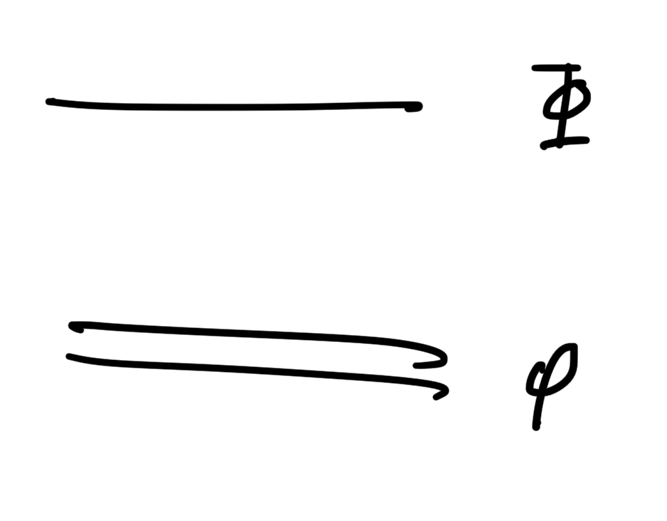
We will denote diagrams using a double line for \( \phi \) and a single line for \( \Phi \), as sketched in

fig. 1. Particle line convention.


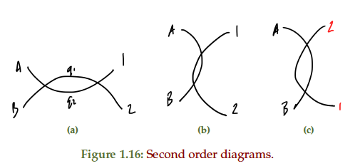
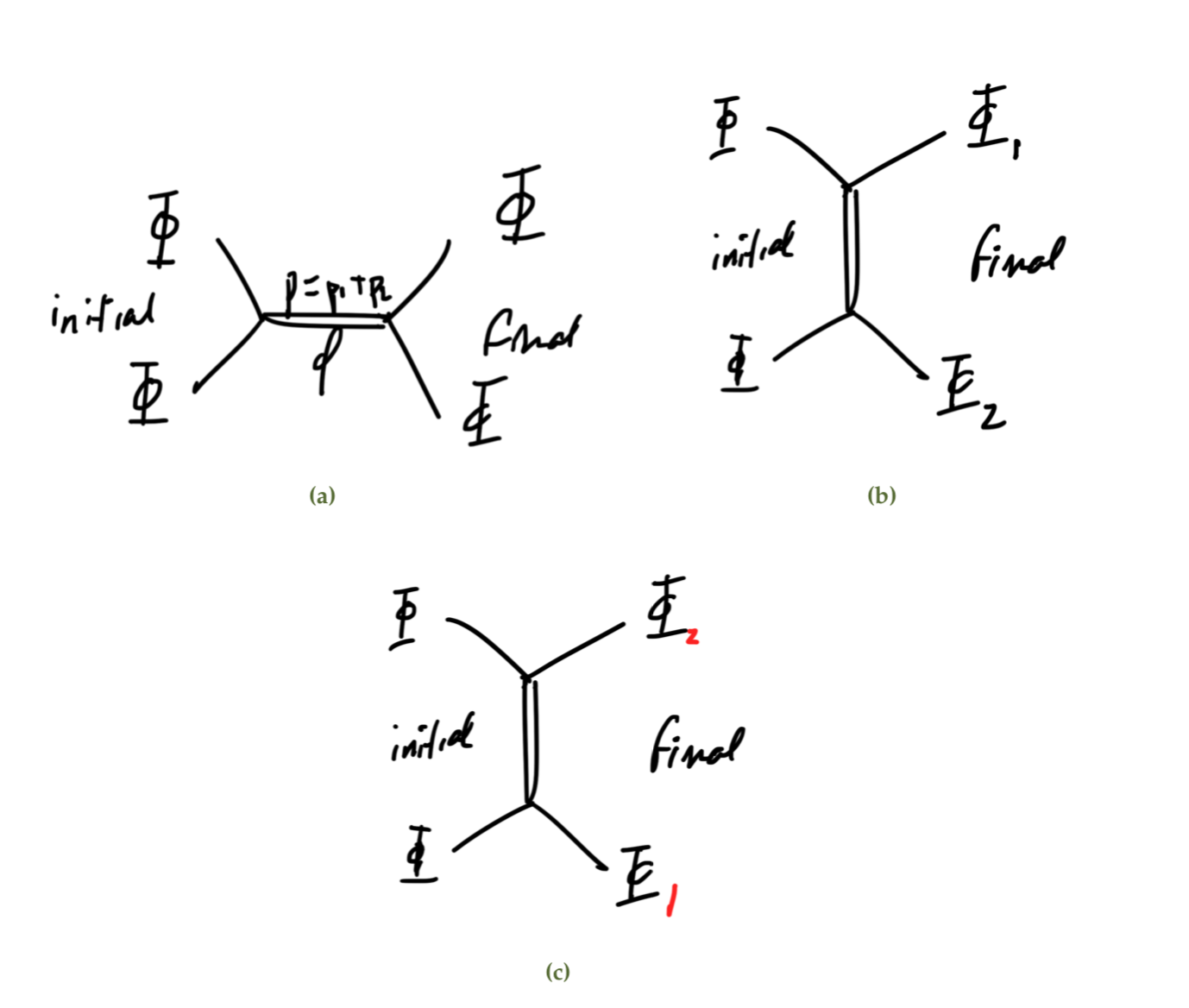
There are three possible diagrams:

fig 2. Possible diagrams.

The first we will call the s-channel, which has amplitude

\begin{equation}\label{eqn:qftLecture17:80}
A(\text{s-channel}) \sim \frac{i}{p^2 – m^2 + i \epsilon} =
\frac{i}{s – m^2 + i \epsilon}
\end{equation}

\begin{equation}\label{eqn:qftLecture17:100}
(p_1 + p_2)^2 = s
\end{equation}
In the centre of mass frame
\begin{equation}\label{eqn:qftLecture17:120}
\Bp_1 = – \Bp_2,
\end{equation}
so
\begin{equation}\label{eqn:qftLecture17:140}
s = \lr{ p_1^0 + p_2^0 }^2 = E_{\text{cm}}^2.
\end{equation}

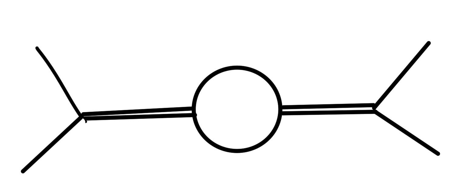
To the next order we have a diagram like fig. 3.

fig. 3. Higher order.

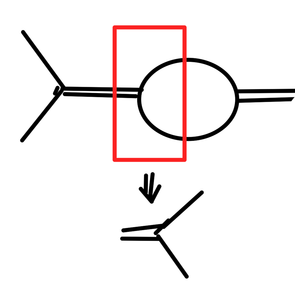
and can have additional virtual particles created, with diagrams like fig. 4.

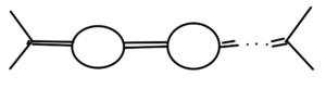
fig. 4. More virtual particles.


We will see (QFT II) that this leads to an addition imaginary \( i \Gamma \) term in the propagator
\begin{equation}\label{eqn:qftLecture17:160}
\frac{i}{s – m^2 + i \epsilon}
\rightarrow
\frac{i}{s – m^2 – i m \Gamma + i \epsilon}.
\end{equation}
If we choose to zoom into the such a figure, as sketched in fig. 5, we find that it contains the interaction of interest for our diagram, so we can (looking forward to currently unknown material) know that our diagram also has such an imaginary \( i \Gamma \) term in its propagator.

fig. 5. Zooming into the diagram for a higher order virtual particle creation event.

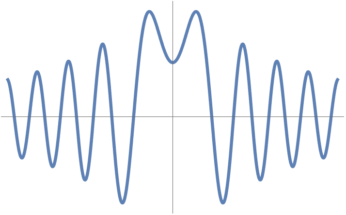
Assuming such a term, the squared amplitude becomes
\begin{equation}\label{eqn:qftLecture17:180}
\evalbar{\sigma}{s \text{near} m^2}
\sim
\Abs{A_s}^2 \sim \inv{(s – m)^2 + m^2 \Gamma^2}
\end{equation}

This is called a resonance (name?), and is sketched in fig. 6.
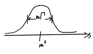
fig. 6. Resonance.


Where are the poles of the modified propagator?

\begin{equation}\label{eqn:qftLecture17:220}
\frac{i}{s – m^2 – i m \Gamma + i \epsilon}
=
\frac{i}{p_0^2 – \Bp^2 – m^2 – i m \Gamma + i \epsilon}
\end{equation}

The pole is found, neglecting \( i \epsilon \), is found at
\begin{equation}\label{eqn:qftLecture17:200}
\begin{aligned}
p_0
&= \sqrt{ \omega_\Bp^2 + i m \Gamma } \\
&= \omega_\Bp \sqrt{ 1 + \frac{i m \Gamma }{\omega_\Bp^2} } \\
&\approx \omega_\Bp + \frac{i m \Gamma }{2 \omega_\Bp}
\end{aligned}
\end{equation}

Decay rates.

We have an initial state
\begin{equation}\label{eqn:qftLecture17:240}
\ket{i} = \ket{k},
\end{equation}
and final state
\begin{equation}\label{eqn:qftLecture17:260}
\ket{f} = \ket{p_1^f, p_2^f \cdots p_n^f}.
\end{equation}
We defined decay rate as the ratio of the number of initial particles to the number of final particles.

The probability is
\begin{equation}\label{eqn:qftLecture17:280}
\rho \sim \Abs{\bra{f} S \ket{i}}^2
=
(2 \pi)^4 \delta^{(4)}( p_{\text{in}} – \sum p_f )
\times \Abs{ M_{fi} }^2
\end{equation}

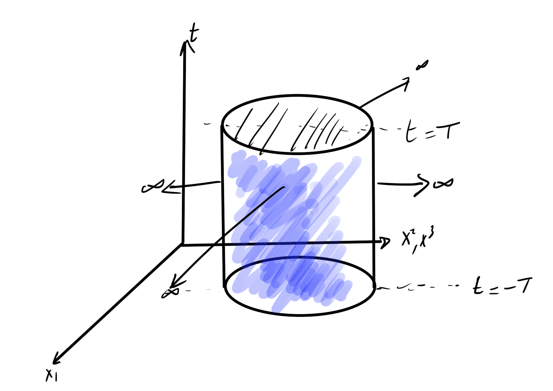
Saying that \( \delta(x) f(x) = \delta(x) f(0) \) we can set the argument of one of the delta functions to zero, which gives us a vacuum volume element factor
\begin{equation}\label{eqn:qftLecture17:300}
(2 \pi)^4
\delta^{(4)}( p_{\text{in}} – \sum p_f ) =
(2 \pi)^4
\delta^{(4)}( 0 )
= V_3 T,
\end{equation}
so
\begin{equation}\label{eqn:qftLecture17:320}
\frac{\text{probability for \( i \rightarrow f\)}}{\text{unit time}}
\sim
(2 \pi)^4 \delta^{(4)}( p_{\text{in}} – \sum p_f )
V_3
\times \Abs{ M_{fi} }^2
\end{equation}

\begin{equation}\label{eqn:qftLecture17:340}
\braket{\Bk}{\Bk} = 2 \omega_\Bk V_3
\end{equation}

coming from

\begin{equation}\label{eqn:qftLecture17:360}
\braket{k}{p} = (2 \pi)^3 2 \omega_\Bp \delta^{(3)}(\Bp – \Bk)
\end{equation}
so
\begin{equation}\label{eqn:qftLecture17:380}
\braket{k}{k} = 2 \omega_\Bp V_3
\end{equation}

\begin{equation}\label{eqn:qftLecture17:400}
\frac{\text{probability for \(i \rightarrow f\)}}{\text{unit time}}
\sim
\frac{
(2 \pi)^4 \delta^{(4)}( p_{\text{in}} – \sum p_f )
\Abs{ M_{fi} }^2 V_3
}
{
2 \omega_\Bk V_3
2 \omega_{\Bp_1}
\cdots
2 \omega_{\Bp_n} V_3^n
}
\end{equation}

If we multiply the number of final states with \( p_i^f \in (p_i^f, p_i^f + dp_i^f) \) for a particle in a box
\begin{equation}\label{eqn:qftLecture17:420}
p_x = \frac{ 2 \pi n_x}{L}
\end{equation}

\begin{equation}\label{eqn:qftLecture17:440}
\Delta p_x = \frac{ 2 \pi }{L} \Delta n_x
\end{equation}

\begin{equation}\label{eqn:qftLecture17:460}
\Delta n_x
=
\frac{L}{2 \pi} \Delta p_x
\end{equation}

and

\begin{equation}\label{eqn:qftLecture17:480}
\Delta n_x
\Delta n_y
\Delta n_z
= \frac{V_3}{(2 \pi)^3 }
\Delta p_x
\Delta p_y
\Delta p_z
\end{equation}

\begin{equation}\label{eqn:qftLecture17:500}
\begin{aligned}
\Gamma
&=
\frac{\text{number of events \( i \rightarrow f \)}}{\text{unit time}} \\
&=
\prod_{f} \frac{ d^3 p}{(2 \pi)^3 2 \omega_{\Bp^f} }
\frac{ (2 \pi)^4 \delta^{(4)}( k – \sum_f p^f ) \Abs{M_{fi}}^2 }
{
2 \omega_{\Bk}
}
\end{aligned}
\end{equation}

Note that everything here is Lorentz invariant except for the denominator of the second term ( \(2 \omega_{\Bk}\)). This is a well known result (the decay rate changes in different frames).

Cross section.

For \( 2 \rightarrow \text{many} \) transitions

\begin{equation}\label{eqn:qftLecture17:520}
\frac{\text{probability \( i \rightarrow f \)}}{\text{unit time}}
\times \lr{
\text{ number of final states with \( p_f \in (p_f, p_f + dp_f) \)
}
}
=
\frac{ (2 \pi)^4 \delta^{(4)}( \sum p_i – \sum_f p^f ) \Abs{M_{fi}}^2 {V_3} }
{
2 \omega_{\Bk_1} V_3
2 \omega_{\Bk_2} {V_3 }
}
\prod_{f} \frac{ d^3 p}{(2 \pi)^3 2 \omega_{\Bp^f} }
\end{equation}

We need to divide by the flux.

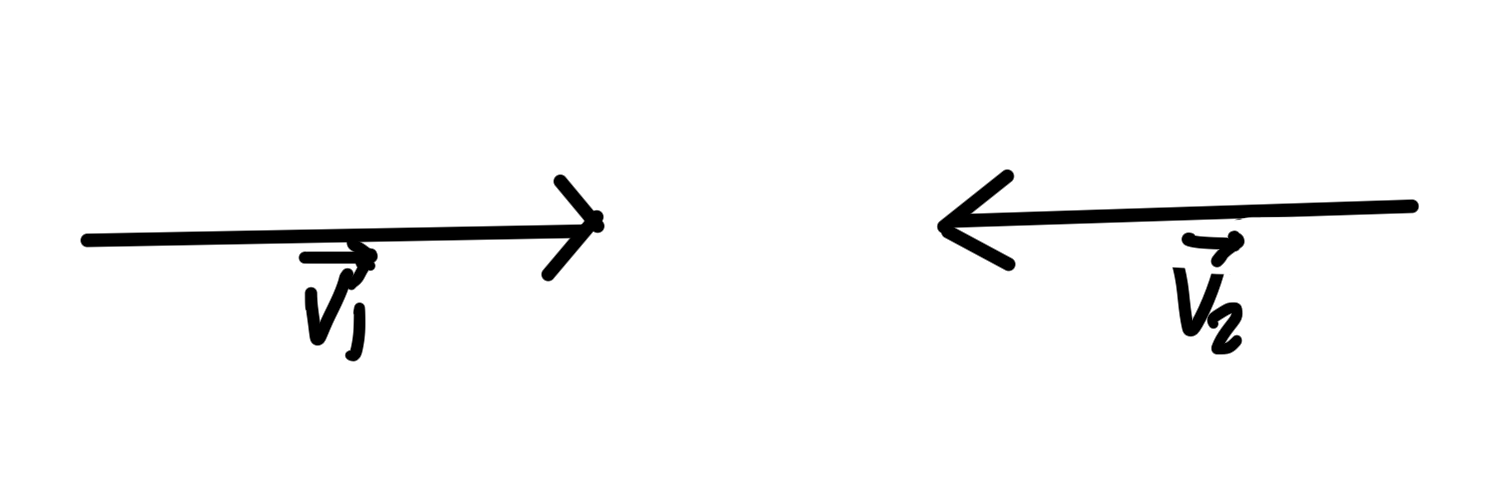
In the CM frame, as sketched in fig. 7, the current is
\begin{equation}\label{eqn:qftLecture17:540}
\Bj = n \Bv_1 – n \Bv_2,
\end{equation}
so if the density is
\begin{equation}\label{eqn:qftLecture17:560}
n = \inv{V_3},
\end{equation}
(one particle in \(V_3\)), then
\begin{equation}\label{eqn:qftLecture17:580}
\Bj = \frac{\Bv_1 – \Bv_2}{V_3}.
\end{equation}

fig. 7. Centre of mass frame.


This is where [1] stops,
\begin{equation}\label{eqn:qftLecture17:640}
\sigma
=
\frac{ (2 \pi)^4 \delta^{(4)}( \sum p_i – \sum_f p^f ) \Abs{M_{fi}}^2 {V_3} }
{
2 \omega_{\Bk_1}
2 \omega_{\Bk_2}
\Abs{\Bv_1 – \Bv_2}
}
\prod_{f} \frac{ d^3 p}{(2 \pi)^3 2 \omega_{\Bp^f} }
\end{equation}

There is, however, a nice Lorentz invariant generalization
\begin{equation}\label{eqn:qftLecture17:600}
j = \inv{ V_3 \omega_{k_A} \omega_{k_B}} \sqrt{ (k_A – k_B)^2 – m_A^2 m_B^2 }
\end{equation}

(Claim: DIY)
\begin{equation}\label{eqn:qftLecture17:620}
\begin{aligned}
\evalbar{j}{CM}
&=
\inv{V_3}
\lr{
\frac{\Abs{\Bk}}{\omega_{k_A}}
+
\frac{\Abs{\Bk}}{\omega_{k_B}}
} \\
&=
\inv{V_3} \lr{ \Abs{\Bv_A} + \Abs{\Bv_B} } \\
&=
\inv{V_3} \Abs{\Bv_1 – \Bv_2 }.
\end{aligned}
\end{equation}

\begin{equation}\label{eqn:qftLecture17:660}
\sigma
=
\frac{ (2 \pi)^4 \delta^{(4)}( \sum p_i – \sum_f p^f ) \Abs{M_{fi}}^2 {V_3} }
{
4 \sqrt{ (k_A – k_B)^2 – m_A^2 m_B^2 }
}
\prod_{f} \frac{ d^3 p}{(2 \pi)^3 2 \omega_{\Bp^f} }.
\end{equation}

References

[1] Michael E Peskin and Daniel V Schroeder. An introduction to Quantum Field Theory. Westview, 1995.

Momentum of scalar field: continued.

November 9, 2018 phy2403 , , , ,

[Click here for a PDF of this post with nicer formatting]

Conservation of the field momentum.

This is a follow up to the unanswered questions I had yesterday related to the apparent time dependent terms in the previous expansion of \( P^i \) for a scalar field.

It turns out that examining the reasons that we can say that the field momentum is conserved also sheds some light on the question. \( P^i \) is not an a-priori conserved quantity, but we may use the charge conservation argument to justify this despite it not having a four-vector nature (i.e. with zero four divergence.)

The momentum \( P^i \) that we have defined is related to the conserved quantity \( T^{0\mu} \), the energy-momentum tensor, which satisfies \( 0 = \partial_\mu T^{0\mu} \) by Noether’s theorem (this was the conserved quantity associated with a spacetime translation.)

That tensor was
\begin{equation}\label{eqn:momentum:120}
T^{\mu\nu} = \partial^\mu \phi \partial^\nu \phi – g^{\mu\nu} \LL,
\end{equation}
and can be used to define the momenta
\begin{equation}\label{eqn:momentum:140}
\begin{aligned}
\int d^3 x T^{0k}
&= \int d^3 x \partial^0 \phi \partial^k \phi \\
&= \int d^3 x \pi \partial^k \phi.
\end{aligned}
\end{equation}
Charge \( Q^i = \int d^3 x j^0 \) was conserved with respect to a limiting surface argument, and we can make a similar “beer can integral” argument for \( P^i \), integrating over a large time interval \( t \in [-T, T] \) as sketched in fig. 1. That is
\begin{equation}\label{eqn:momentum:160}
\begin{aligned}
0
&=
\partial_\mu \int d^4 x T^{0\mu} \\
&=
\partial_0 \int d^4 x T^{00}
+
\partial_k \int d^4 x T^{0k} \\
&=
\partial_0 \int_{-T}^T dt \int d^3 x T^{00}
+
\partial_k \int_{-T}^T dt \int d^3 x T^{0k} \\
&=
\partial_0 \int_{-T}^T dt \int d^3 x T^{00}
+
\partial_k \int_{-T}^T dt
\inv{2} \int \frac{d^3 p }{(2 \pi)^3} p^k
\lr{
a_\Bp^\dagger a_\Bp
+ a_\Bp a_\Bp^\dagger
– a_\Bp a_{-\Bp} e^{- 2 i \omega_\Bp t}
– a_\Bp^\dagger a_{-\Bp}^\dagger e^{2 i \omega_\Bp t}
} \\
&=
\int d^3 x \evalrange{T^{00}}{-T}{T}
+
T \partial_k
\int \frac{d^3 p }{(2 \pi)^3} p^k
\lr{
a_\Bp^\dagger a_\Bp
+ a_\Bp a_\Bp^\dagger
}
-\inv{2}
\partial_k \int_{-T}^T dt
\int \frac{d^3 p }{(2 \pi)^3} p^k
\lr{
a_\Bp a_{-\Bp} e^{- 2 i \omega_\Bp t}
+ a_\Bp^\dagger a_{-\Bp}^\dagger e^{2 i \omega_\Bp t}
}.
\end{aligned}
\end{equation}

fig. 1. Cylindrical spacetime boundary.

The first integral can be said to vanish if the field energy goes to zero at the time boundaries, and the last integral reduces to
\begin{equation}\label{eqn:momentum:180}
\begin{aligned}
-\inv{2}
\partial_k \int_{-T}^T dt
\int \frac{d^3 p }{(2 \pi)^3} p^k
\lr{
a_\Bp a_{-\Bp} e^{- 2 i \omega_\Bp t}
+ a_\Bp^\dagger a_{-\Bp}^\dagger e^{2 i \omega_\Bp t}
}
&=
-\int \frac{d^3 p }{2 (2 \pi)^3} p^k
\lr{
a_\Bp a_{-\Bp} \frac{\sin( -2 \omega_\Bp T )}{-2 \omega_\Bp}
+ a_\Bp^\dagger a_{-\Bp}^\dagger \frac{\sin( 2 \omega_\Bp T )}{2 \omega_\Bp}
} \\
&=
-\int \frac{d^3 p }{2 (2 \pi)^3} p^k
\lr{
a_\Bp a_{-\Bp} + a_\Bp^\dagger a_{-\Bp}^\dagger
}
\frac{\sin( 2 \omega_\Bp T )}{2 \omega_\Bp}
.
\end{aligned}
\end{equation}
The \( \sin \) term can be interpretted as a sinc like function of \( \omega_\Bp \) which vanishes for large \( \Bp \). It’s not entirely sinc like for a massive field as \( \omega_\Bp = \sqrt{ \Bp^2 + m^2 } \), which never hits zero, as shown in fig. 2.

fig 2. sin(2 omega T)/omega

Vanishing for large \( \Bp \) doesn’t help the whole integral vanish, but we can resort to the Riemann-Lebesque lemma [1] instead and interpret this integral as one with a plain old high frequency oscillation that is presumed to vanish (i.e. the rest is well behaved enough that it can be labelled as \( L_1 \) integrable.)

We see that only the non-time dependent portion of \( \mathbf{P} \) matters from a conserved quantity point of view, and having killed off all the time dependent terms, we are left with a conservation relationship for the momenta \( \spacegrad \cdot \BP = 0 \), where \( \BP \) in normal order is just
\begin{equation}\label{eqn:momentum:200}
: \BP : = \int \frac{d^3 p}{(2 \pi)^3} \Bp a_\Bp^\dagger a_\Bp.
\end{equation}

References

[1] Wikipedia contributors. Riemann-lebesgue lemma — Wikipedia, the free encyclopedia, 2018. URL https://en.wikipedia.org/w/index.php?title=Riemann%E2%80%93Lebesgue_lemma&oldid=856778941. [Online; accessed 29-October-2018].

PHY2403: QFT I: Momentum of scalar field: time dependent terms?

November 8, 2018 phy2403 , , ,

[Click here for a PDF of this post with nicer formatting]

Way back in lecture 8, it was claimed that
\begin{equation}\label{eqn:momentum:20}
P^k = \int d^3 x \hat{\pi} \partial^k \hat{\phi} = \int \frac{d^3 p}{(2\pi)^3} p^k a_\Bp^\dagger a_\Bp.
\end{equation}
If I compute this, I get a normal ordered variation of this operator, but also get some time dependent terms. Here’s the computation (dropping hats)
\begin{equation}\label{eqn:momentum:40}
\begin{aligned}
P^k
&= \int d^3 x \hat{\pi} \partial^k \phi \\
&= \int d^3 x \partial_0 \phi \partial^k \phi \\
&= \int d^3 x \frac{d^3 p d^3 q}{(2 \pi)^6} \inv{\sqrt{2 \omega_p 2 \omega_q} }
\partial_0
\lr{
a_\Bp e^{-i p \cdot x}
+
a_\Bp^\dagger e^{i p \cdot x}
}
\partial^k
\lr{
a_\Bq e^{-i q \cdot x}
+
a_\Bq^\dagger e^{i q \cdot x}
}.
\end{aligned}
\end{equation}
The exponential derivatives are
\begin{equation}\label{eqn:momentum:60}
\begin{aligned}
\partial_0 e^{\pm i p \cdot x}
&=
\partial_0 e^{\pm i p_\mu x^\mu} \\
&=
\pm i p_0
\partial_0 e^{\pm i p \cdot x},
\end{aligned}
\end{equation}
and
\begin{equation}\label{eqn:momentum:80}
\begin{aligned}
\partial^k e^{\pm i p \cdot x}
&=
\partial^k e^{\pm i p^\mu x_\mu} \\
&=
\pm i p^k e^{\pm i p \cdot x},
\end{aligned}
\end{equation}
so
\begin{equation}\label{eqn:momentum:100}
\begin{aligned}
P^k
&=
-\int d^3 x \frac{d^3 p d^3 q}{(2 \pi)^6} \inv{\sqrt{2 \omega_p 2 \omega_q} }
p_0 q^k
\lr{
-a_\Bp e^{-i p \cdot x}
+
a_\Bp^\dagger e^{i p \cdot x}
}
\lr{
-a_\Bq e^{-i q \cdot x}
+
a_\Bq^\dagger e^{i q \cdot x}
} \\
&=
-\inv{2} \int d^3 x \frac{d^3 p d^3 q}{(2 \pi)^6} \sqrt{\frac{\omega_p}{\omega_q}} q^k
\lr{
a_\Bp a_\Bq e^{-i (p + q) \cdot x}
+ a_\Bp^\dagger a_\Bq^\dagger e^{i (p + q) \cdot x}
– a_\Bp a_\Bq^\dagger e^{i (q – p) \cdot x}
– a_\Bp^\dagger a_\Bq e^{i (p – q) \cdot x}
} \\
&=
\inv{2} \int \frac{d^3 p d^3 q}{(2 \pi)^3} \sqrt{\frac{\omega_p}{\omega_q}} q^k
\lr{
– a_\Bp a_\Bq e^{- i(\omega_\Bp + \omega_\Bq) t} \delta^3(\Bp + \Bq)
– a_\Bp^\dagger a_\Bq^\dagger e^{i(\omega_\Bp + \omega_\Bq) t} \delta^3(-\Bp – \Bq)
+ a_\Bp a_\Bq^\dagger e^{i(\omega_\Bq – \omega_\Bp) t} \delta^3(\Bp – \Bq)
+ a_\Bp^\dagger a_\Bq e^{i(\omega_\Bp – \omega_\Bq) t} \delta^3(\Bq – \Bp)
} \\
&=
\inv{2} \int \frac{d^3 p }{(2 \pi)^3} p^k
\lr{
a_\Bp^\dagger a_\Bp
+ a_\Bp a_\Bp^\dagger
– a_\Bp a_{-\Bp} e^{- 2 i \omega_\Bp t}
– a_\Bp^\dagger a_{-\Bp}^\dagger e^{2 i \omega_\Bp t}
}.
\end{aligned}
\end{equation}

What is the rationale for ignoring those time dependent terms? Does normal ordering also implicitly drop any non-paired creation/annihilation operators? If so, why?