References

[Click here for a PDF of this post with nicer formatting]

An incorrect start at a field theory problem.

The following is a problem from the second PHY2403 problem set, and the start of a solution attempt I made. I’m not posting this because it shows how to do the problem, but because it was a useful problem to show that I didn’t understand a lot of the problem statement.
Understanding where I went wrong is actually pretty useful in this case.

Problem: Playing with the non-relativistic limit

Consider a real scalar relativistic field theory of mass m with \( \lambda \phi^4 \) interaction. Let there be \( N \) particles of momenta labeled by \( p_1,\cdots, p_N\), whose energies are such that they are insufficient to create any new particles. Nevertheless, the particles can scatter and exchange momenta. In what follows you will study this N-particle nonrelativistic limit in some detail.

1. Write down the Hamiltonian of the field theory, including the interaction term, restricted to the N-particle sector of Hilbert space. (Use the creation and annihilation operator representation, i.e. write the result as sums of products of creation and annihilation operators of particles of various momenta.)
2. Does the resulting Hamiltonian preserve particle number? Is there an associated symmetry? What is the operator that generates it?
3. Consider now the interaction term in your reduced (to the N-particle sector of Hilbert space) Hamiltonian. How does a typical interaction term (for given configurations of momenta) act on an N-particle state? What kinds of scattering processes does it describe?
4. What do you think is the potential, in x-space, that allows the various particles to scatter and exchange momentum? How would you describe the resulting nonrelativistic quantum system to friends who never took QFT but are well-versed in quantum mechanics?

Incorrect answer attempt.

The Lagrangian density of a massive scalar field with a \( \lambda \phi^4 \) interaction has the form
\begin{equation}\label{eqn:Nparticle:20}
\LL = \inv{2} \partial_\mu \phi \partial^\mu \phi – \inv{2} m^2 \phi^2 – \lambda \phi^4.
\end{equation}
The corresponding Hamiltonian is
\begin{equation}\label{eqn:Nparticle:40}
H = \inv{2} \int d^3x \lr{ \pi^2 + \frac{m^2}{2} (\spacegrad \phi)^2 + m^2 \phi^2 } + \lambda \int d^3 x \phi^4.
\end{equation}
In terms of creation and annihilation operators, we know the form of the non-interaction portion of the Hamiltonian, which in normal order is
\begin{equation}\label{eqn:Nparticle:60}
H_0 = \int \frac{d^3 p}{(2 \pi)^3} \omega_\Bp a_\Bp^\dagger a_\Bp,
\end{equation}
but the interaction contribution is much messier
\begin{equation}\label{eqn:Nparticle:80}
\begin{aligned}
H_{\text{int}}
&=
\lambda \int d^3 x \frac{ d^3 p d^3 k d^3 q d^3 s}{4 (2 \pi)^{12} \sqrt{
\omega_\Bp \omega_\Bk \omega_\Bq \omega_\Bs
} }
\lr{ a_\Bp e^{-i p \cdot x} + a_\Bp e^{i p \cdot x} }
\lr{ a_\Bk e^{-i k \cdot x} + a_\Bk e^{i k \cdot x} }
\lr{ a_\Bq e^{-i q \cdot x} + a_\Bq e^{i q \cdot x} }
\lr{ a_\Bs e^{-i s \cdot x} + a_\Bs e^{i s \cdot x} } \\
&=
\lambda \int d^3 x \frac{ d^3 p d^3 k d^3 q d^3 s}{4 (2 \pi)^{12} \sqrt{
\omega_\Bp \omega_\Bk \omega_\Bq \omega_\Bs
} }
\lr{ a_\Bp e^{-i \omega_\Bp t + i \Bp \cdot \Bx} + a_\Bp e^{i \omega_\Bp t – i \Bp \cdot \Bx} }
\lr{ a_\Bk e^{-i \omega_\Bk t + i \Bk \cdot \Bx} + a_\Bk e^{i \omega_\Bk t – i \Bk \cdot \Bx} } \\
&\quad \lr{ a_\Bq e^{-i \omega_\Bq t + i \Bq \cdot \Bx} + a_\Bq e^{i \omega_\Bq t – i \Bq \cdot \Bx} }
\lr{ a_\Bs e^{-i \omega_\Bs t + i \Bs \cdot \Bx} + a_\Bs e^{i \omega_\Bs t – i \Bs \cdot \Bx} } \\
&=
\lambda \int \frac{ d^3 p d^3 k d^3 q d^3 s}{4 (2 \pi)^{9} \sqrt{
\omega_\Bp \omega_\Bk \omega_\Bq \omega_\Bs
} }
\Big(
a_\Bp a_\Bk a_\Bq a_\Bs e^{-i (\omega_\Bp + \omega_\Bk + \omega_\Bq + \omega_\Bs)t} \delta^3( \Bp + \Bk + \Bq + \Bs ) \\
&\qquad +
a_\Bp a_\Bk a_\Bq a_\Bs^\dagger e^{-i (\omega_\Bp + \omega_\Bk + \omega_\Bq – \omega_\Bs)t} \delta^3( \Bp + \Bk + \Bq – \Bs ) \\
&\qquad \\
&\qquad + \cdots \\
&\qquad +
a_\Bp^\dagger a_\Bk^\dagger a_\Bq^\dagger a_\Bs^\dagger e^{-i (-\omega_\Bp – \omega_\Bk – \omega_\Bq – \omega_\Bs)t} \delta^3( -\Bp – \Bk – \Bq – \Bs )
\Big) \\
&=
\lambda \int \frac{ d^3 p d^3 k d^3 q }{4 (2 \pi)^{9}
}
\Big(
\inv{\sqrt{
\omega_\Bp \omega_\Bk \omega_\Bq \omega_{-\Bp – \Bk – \Bq}
}}
a_\Bp a_\Bk a_\Bq a_{-\Bp -\Bk – \Bq} e^{-i (\omega_\Bp + \omega_\Bk + \omega_\Bq + \omega_{-\Bp -\Bk -\Bq})t} \\
&\qquad +
\inv{\sqrt{
\omega_\Bp \omega_\Bk \omega_\Bq \omega_{\Bp + \Bk + \Bq}
}}
a_\Bp a_\Bk a_\Bq a_{\Bp + \Bk + \Bq}^\dagger e^{-i (\omega_\Bp + \omega_\Bk + \omega_\Bq – \omega_{\Bp + \Bk + \Bq})t} \\
&\qquad +
\cdots \\
&\qquad +
\inv{\sqrt{
\omega_\Bp \omega_\Bk \omega_\Bq \omega_{-\Bp – \Bk – \Bq}
}}
a_\Bp^\dagger a_\Bk^\dagger a_\Bq^\dagger a_{-\Bp -\Bk -\Bq}^\dagger e^{-i (-\omega_\Bp – \omega_\Bk – \omega_\Bq – \omega_{-\Bp -\Bk -\Bq})t}
\Big)
\end{aligned}
\end{equation}
Assuming we can normal order these terms as in \( H_0 \), we can rewrite the interaction as
\begin{equation}\label{eqn:Nparticle:100}
\begin{aligned}
H_{\text{int}}
&=
\lambda \int \frac{ d^3 p d^3 k d^3 q }{4 (2 \pi)^{9} }
\Big(
\binom{4}{0}
\inv{\sqrt{
\omega_\Bp \omega_\Bk \omega_\Bq \omega_{-\Bp – \Bk – \Bq}
}}
a_\Bp a_\Bk a_\Bq a_{-\Bp -\Bk – \Bq} e^{-i (\omega_\Bp + \omega_\Bk + \omega_\Bq + \omega_{-\Bp -\Bk -\Bq})t} \\
&\qquad +
\binom{4}{1}
\inv{\sqrt{
\omega_\Bp \omega_\Bk \omega_\Bq \omega_{\Bp – \Bk – \Bq}
}}
a_\Bp^\dagger a_\Bk a_\Bq a_{\Bp – \Bk – \Bq} e^{-i (-\omega_\Bp + \omega_\Bk + \omega_\Bq + \omega_{\Bp – \Bk – \Bq})t} \\
&\qquad +
\binom{4}{2}
\inv{\sqrt{
\omega_\Bp \omega_\Bk \omega_\Bq \omega_{\Bp + \Bk – \Bq}
}}
a_\Bp^\dagger a_\Bk^\dagger a_\Bq a_{\Bp + \Bk – \Bq} e^{-i (-\omega_\Bp – \omega_\Bk + \omega_\Bq + \omega_{\Bp + \Bk – \Bq})t} \\
&\qquad +
\binom{4}{3}
\inv{\sqrt{
\omega_\Bp \omega_\Bk \omega_\Bq \omega_{\Bp + \Bk _ \Bq}
}}
a_\Bp^\dagger a_\Bk^\dagger a_\Bq^\dagger a_{\Bp + \Bk + \Bq} e^{-i (-\omega_\Bp – \omega_\Bk – \omega_\Bq + \omega_{\Bp + \Bk + \Bq})t} \\
&\qquad +
\binom{4}{4}
\inv{\sqrt{
\omega_\Bp \omega_\Bk \omega_\Bq \omega_{-\Bp – \Bk – \Bq}
}}
a_\Bp^\dagger a_\Bk^\dagger a_\Bq^\dagger a_{-\Bp -\Bk -\Bq}^\dagger e^{-i (-\omega_\Bp – \omega_\Bk – \omega_\Bq – \omega_{-\Bp -\Bk -\Bq})t}
\Big)
\end{aligned}
\end{equation}

If we restrict the allowed momenta to the discrete set \( \Bp \in \setlr{ \Bp_1, \Bp_2, \cdots \Bp_N} \), the total Hamiltonian including the interaction term
takes the form
\begin{equation}\label{eqn:Nparticle:120}
\begin{aligned}
\text{\(:H:\)} &=
\sum_{i = 1}^N \omega_{\Bp_i} a_{\Bp_i}^\dagger a_{\Bp_i}
+
\frac{
\lambda
}{4 }
\sum_{j,m,n = 1}^N
\Big(
\binom{4}{0}
\inv{\sqrt{
\omega_{\Bp_j} \omega_{\Bp_m} \omega_{\Bp_n} \omega_{-{\Bp_j} – {\Bp_m} – {\Bp_n}}
}}
a_{\Bp_j} a_{\Bp_m} a_{\Bp_n} a_{-\Bp -\Bk – \Bq} e^{-i (\omega_{\Bp_j} + \omega_{\Bp_m} + \omega_{\Bp_n} + \omega_{-{\Bp_j} -{\Bp_m} -{\Bp_n}})t} \\
&\qquad +
\binom{4}{1}
\inv{\sqrt{
\omega_{\Bp_j} \omega_{\Bp_m} \omega_{\Bp_n} \omega_{{\Bp_j} – {\Bp_m} – {\Bp_n}}
}}
a_{\Bp_j}^\dagger a_{\Bp_m} a_{\Bp_n} a_{{\Bp_j} – {\Bp_m} – {\Bp_n}} e^{-i (-\omega_{\Bp_j} + \omega_{\Bp_m} + \omega_{\Bp_n} + \omega_{{\Bp_j} – {\Bp_m} – {\Bp_n}})t} \\
&\qquad +
\binom{4}{2}
\inv{\sqrt{
\omega_{\Bp_j} \omega_{\Bp_m} \omega_{\Bp_n} \omega_{{\Bp_j} + {\Bp_m} – {\Bp_n}}
}}
a_{\Bp_j}^\dagger a_{\Bp_m}^\dagger a_{\Bp_n} a_{{\Bp_j} + {\Bp_m} – {\Bp_n}} e^{-i (-\omega_{\Bp_j} – \omega_{\Bp_m} + \omega_{\Bp_n} + \omega_{{\Bp_j} + {\Bp_m} – {\Bp_n}})t} \\
&\qquad +
\binom{4}{3}
\inv{\sqrt{
\omega_{\Bp_j} \omega_{\Bp_m} \omega_{\Bp_n} \omega_{{\Bp_j} + {\Bp_m} – {\Bp_n}}
}}
a_{\Bp_j}^\dagger a_{\Bp_m}^\dagger a_{\Bp_n}^\dagger a_{{\Bp_j} + {\Bp_m} + {\Bp_n}} e^{-i (-\omega_{\Bp_j} – \omega_{\Bp_m} – \omega_{\Bp_n} + \omega_{{\Bp_j} + {\Bp_m} + {\Bp_n}})t} \\
&\qquad +
\binom{4}{4}
\inv{\sqrt{
\omega_{\Bp_j} \omega_{\Bp_m} \omega_{\Bp_n} \omega_{-{\Bp_j} – {\Bp_m} – {\Bp_n}}
}}
a_{\Bp_j}^\dagger a_{\Bp_m}^\dagger a_{\Bp_n}^\dagger a_{-{\Bp_j} -{\Bp_m} -{\Bp_n}}^\dagger e^{-i (-\omega_{\Bp_j} – \omega_{\Bp_m} – \omega_{\Bp_n} – \omega_{-{\Bp_j} -{\Bp_m} -{\Bp_n}})t}
\Big)
\end{aligned}
\end{equation}

When we did the same sort of calculation for \( (\spacegrad \phi)^2 + m^2 \phi^2 \) all the time dependent terms cancelled nicely, but that isn’t obviously the case here.
However, we haven’t used the non-relativistic (low energy) constraint. That constraint can be expressed as \( \Bp^2 \ll m^2 \), in which case \( \omega_\Bp = \sqrt{ \Bp^2 + m^2 } \sim m \), the mass of each of the particles. Incorporating that into our N-particle Hamiltonian, we have
\begin{equation}\label{eqn:Nparticle:140}
\begin{aligned}
\text{\(:H:\)} &=
\sum_{i = 1}^N \omega_{\Bp_i} a_{\Bp_i}^\dagger a_{\Bp_i}
+
\frac{
\lambda
}{4 m^2 }
\sum_{j,m,n = 1}^N
\Big(
\binom{4}{0}
a_{\Bp_j} a_{\Bp_m} a_{\Bp_n} a_{-\Bp -\Bk – \Bq} e^{- 4 i m t} \\
&\qquad +
\binom{4}{1}
a_{\Bp_j}^\dagger a_{\Bp_m} a_{\Bp_n} a_{{\Bp_j} – {\Bp_m} – {\Bp_n}} e^{-3 i m t} \\
&\qquad +
\binom{4}{2}
a_{\Bp_j}^\dagger a_{\Bp_m}^\dagger a_{\Bp_n} a_{{\Bp_j} + {\Bp_m} – {\Bp_n}} \\
&\qquad +
\binom{4}{3}
a_{\Bp_j}^\dagger a_{\Bp_m}^\dagger a_{\Bp_n}^\dagger a_{{\Bp_j} + {\Bp_m} + {\Bp_n}} e^{ 3 i m t } \\
&\qquad +
\binom{4}{4}
a_{\Bp_j}^\dagger a_{\Bp_m}^\dagger a_{\Bp_n}^\dagger a_{-{\Bp_j} -{\Bp_m} -{\Bp_n}}^\dagger e^{4 i m t}
\Big).
\end{aligned}
\end{equation}

The only annoying aspect to this Hamiltonian is the \( a_{{\Bp_j} + {\Bp_m} – {\Bp_n}} \) operator in the interaction term, which is not clear to me how to interpret. That seems to imply that it is possible to create particles with linear combinations of momentum that may not be in the original set of \( N \) particle momenta. I think that this can be further fudged by invoking the non-relativistic constraint again, and decreeing that each of the uniquely indexed creation and annihilation operators are distinguishable only by index, so we can write the N-particle non-relativistic sector Hamiltonian as
\begin{equation}\label{eqn:Nparticle:170}
\text{\(:H:\)} =
\sum_{i = 1}^N \omega_{\Bp_i}
a_{i}^\dagger a_{i}
+
\frac{
3 \lambda
}{2 m^2 }
\sum_{r,s,t,u = 1}^N
a_{r}^\dagger a_{s}^\dagger a_{t} a_{u}.
\end{equation}

Commentary.

While there are a few things that are not wrong above, those correct parts are liberally mixed with a few fundamental errors.

Even before getting to the fundamential errors, there are a few minor issues too. For example, I don’t think that there is anything strictly wrong with the expansion of \ref{eqn:Nparticle:100} for example, although it appears that I confused myself by actually evaluating the delta function instead of just identifying it, something like:
\begin{equation}\label{eqn:Nparticle:190}
\begin{aligned}
H_{\text{int}}
&=
\frac{\lambda}{4} \int \frac{ d^3 p d^3 k d^3 q d^3 s}{(2 \pi)^{12} \sqrt{ \omega_\Bp \omega_\Bk \omega_\Bq \omega_\Bs } }
\Big(
\binom{4}{0}
\delta^3( \Bp + \Bk + \Bq + \Bs )
a_\Bp a_\Bk a_\Bq a_\Bs e^{-i (\omega_\Bp + \omega_\Bk + \omega_\Bq + \omega_\Bs) t} \\
&\qquad +
\binom{4}{1}
\delta^3( -\Bp + \Bk + \Bq + \Bs )
a_\Bp^\dagger a_\Bk a_\Bq a_\Bs e^{-i (-\omega_\Bp + \omega_\Bk + \omega_\Bq + \omega_\Bs)t} \\
&\qquad +
\binom{4}{2}
\delta^3( -\Bp – \Bk + \Bq + \Bs )
a_\Bp^\dagger a_\Bk^\dagger a_\Bq a_\Bs e^{-i (-\omega_\Bp – \omega_\Bk + \omega_\Bq + \omega_\Bs)t} \\
&\qquad +
\binom{4}{3}
\delta^3( -\Bp – \Bk – \Bq + \Bs )
a_\Bp^\dagger a_\Bk^\dagger a_\Bq^\dagger a_\Bs e^{-i (-\omega_\Bp – \omega_\Bk – \omega_\Bq + \omega_\Bs)t} \\
&\qquad +
\binom{4}{4}
\delta^3( -\Bp – \Bk – \Bq – \Bs )
a_\Bp^\dagger a_\Bk^\dagger a_\Bq^\dagger a_\Bs^\dagger e^{-i (-\omega_\Bp – \omega_\Bk – \omega_\Bq – \omega_\Bs)t}
\Big)
\end{aligned}
\end{equation}

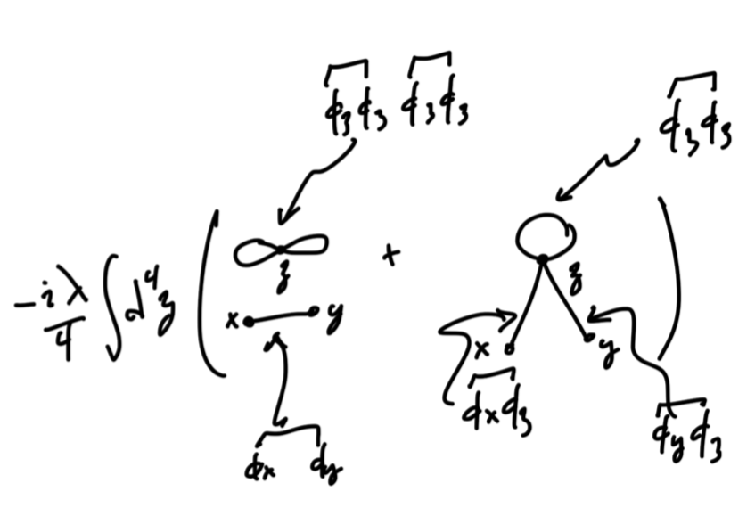
So much of QFT is expressed in terms of delta functions, yet I tend to view them as something to be eliminated instead of retained. One lesson is that delta functions in QFT should be embraced, and had I done so in this case, I would have had a better chance of understanding the scattering part of the question that came later. One role of the delta function actually appears to be critical to the scattering question, as it actually encodes the constraints that lead to conservation of momentum in a “scattering process” related to the interaction term of the Hamiltonian.

I didn’t understand what was meant by a scattering process, but that was related to another more fundamental misunderstanding. That screw up was in my interpretation of what was meant by the “N particle sector of the Hilbert space.” In my reading of that phrase I tossed out “Hilbert space” as irrelevant. Part of that was somewhat reactionary, as it seems to me that Hilbert space is tossed around in so much QM in a way that makes it seem more rigorous, but we never touch on the scary mathematics that rigorously defines what a Hilbert space is. It seems to me that the phrase “Hilbert space” is often used as a pretentious way of saying “complex inner product space”. It has a more precise meaning to Mathematicians, but I don’t think that most physicists understand that meaning (and most certainly most students of QM don’t).

So, long story short, I interpreted “N particle sector of the Hilbert space” as “N particle sector” and though that meant I had to somehow discretize the system, introducing N discrete momenta into the mix. Here’s an example, using the non-interaction Hamiltonian, of exactly how I did that:
\begin{equation}\label{eqn:Nparticle:210}
\int \frac{d^3 p}{(2 \pi)^3} \omega_\Bp a_\Bp^\dagger a_\Bp \rightarrow \sum_{i = 1}^N \omega_\Bp a_\Bp^\dagger a_\Bp.
\end{equation}

This is wrong! I actually clued into part of the trouble with this, but didn’t know what the root cause was. I fudged around that my dropping the problematic side effects of having evaluated the delta function, which lead me to have terms like \( a_{\Bp + \Bq – \Bk} \) in the expansion of the interaction Hamiltonian. I couldn’t see how creation and annihilation operators that are associated with arbitrary linear combinations of the other momenta could maintain an \( N \) particle system. Those linear combinations could easily lie outside of the set of the original \( N \) particle system that I constructed in my discretization.

In office hours, Professor Poppitz had me work a small problem to illustrate the error in my ways, specifically applying the Hamiltonian to a two momentum state
\begin{equation}\label{eqn:Nparticle:230}
\begin{aligned}
H \ket{\Bp_1 \Bp_2}
&=
\lr{
\int \frac{d^3}{(2 \pi)^3}
a_\Bp^\dagger
a_\Bp
}
a_{\Bp_1}^\dagger
a_{\Bp_2}^\dagger
\ket{0} \\
&=
\int \frac{d^3}{(2 \pi)^3} \omega_\Bp
a_\Bp^\dagger
\lr{
a_{\Bp_1}^\dagger a_\Bp
+ (2 \pi) \delta^3(\Bp -\Bp_1)
}
a_{\Bp_2}^\dagger
\ket{0} \\
&=
\int \frac{d^3}{(2 \pi)^3} \omega_\Bp
a_\Bp^\dagger
a_{\Bp_1}^\dagger a_\Bp
a_{\Bp_2}^\dagger
\ket{0}
+
\omega_{\Bp_1}
a_{\Bp_1}^\dagger
a_{\Bp_2}^\dagger
\ket{0} \\
&=
\int \frac{d^3}{(2 \pi)^3} \omega_\Bp
a_\Bp^\dagger
a_{\Bp_1}^\dagger
\lr{
a_{\Bp_2}^\dagger
a_\Bp
+ (2 \pi)^3 \delta^3(\Bp – \Bp_2)
}
\ket{0}
+
\omega_{\Bp_1}\ket{\Bp_1 \Bp_2} \\
&=
\lr{ \omega_{\Bp_1} + \omega_{\Bp_2} }
\ket{\Bp_1 \Bp_2}.
\end{aligned}
\end{equation}
Observe that the Hamiltonian operates on a two momentum state, returning that state scaled by the energy associated with the sum of the momenta. Given an two particle subspace of all the possible two momentum states, perhaps with a basis like \( \setlr{\ket{\Bp_1 \Bp_2}, \ket{\Bp_3 \Bp_4}, \cdots } \), the Hamiltonian provides a mapping from that set onto itself, as it scales the states in question, but does not convert two particle states into combinations of one and three momentum states (say). This is not the case with the interaction Hamiltonian, as an operation like \( \int a^\dagger a^\dagger a^\dagger a \) doesn’t preserve a two momentum state. Example
\begin{equation}\label{eqn:Nparticle:250}
\begin{aligned}
\int
&\frac{d^3 p}{(2\pi)^3\sqrt{ 2\omega_\Bp}}
\frac{d^3 q}{(2\pi)^3\sqrt{ 2\omega_\Bq}}
\frac{d^3 r}{(2\pi)^3\sqrt{ 2\omega_\Br}}
\frac{d^3 s}{(2\pi)^3\sqrt{ 2\omega_\Bs}}
\delta^3(\Bp + \Bq + \Br -\Bs)
a_\Bp^\dagger
a_\Bq^\dagger
a_\Br^\dagger
a_\Bs
\ket{ \Bp_1 \Bp_2 } \\
&=
\int
\frac{d^3 p}{(2\pi)^3\sqrt{ 2\omega_\Bp}}
\frac{d^3 q}{(2\pi)^3\sqrt{ 2\omega_\Bq}}
\frac{d^3 r}{(2\pi)^3\sqrt{ 2\omega_\Br}}
\frac{d^3 s}{(2\pi)^3\sqrt{ 2\omega_\Bs}}
\delta^3(\Bp + \Bq + \Br -\Bs)
a_\Bp^\dagger
a_\Bq^\dagger
a_\Br^\dagger
a_\Bs
a_{\Bp_1}^\dagger
a_{\Bp_2}^\dagger
\ket{0} \\
&=
\int
\frac{d^3 p}{(2\pi)^3\sqrt{ 2\omega_\Bp}}
\frac{d^3 q}{(2\pi)^3\sqrt{ 2\omega_\Bq}}
\frac{d^3 r}{(2\pi)^3\sqrt{ 2\omega_\Br}}
\frac{d^3 s}{(2\pi)^3\sqrt{ 2\omega_\Bs}}
\delta^3(\Bp + \Bq + \Br -\Bs)
a_\Bp^\dagger
a_\Bq^\dagger
a_\Br^\dagger
\lr{
a_{\Bp_1}^\dagger
a_\Bs
+ (2 \pi)^3 \delta^3(\Bp_1 -\Bs)
}
a_{\Bp_2}^\dagger
\ket{0} \\
&=
\int
\frac{d^3 p}{(2\pi)^3\sqrt{ 2\omega_\Bp}}
\frac{d^3 q}{(2\pi)^3\sqrt{ 2\omega_\Bq}}
\frac{d^3 r}{(2\pi)^3\sqrt{ 2\omega_\Br}}
\frac{d^3 s}{(2\pi)^3\sqrt{ 2\omega_\Bs}}
\delta^3(\Bp + \Bq + \Br -\Bs)
a_\Bp^\dagger
a_\Bq^\dagger
a_\Br^\dagger
a_{\Bp_1}^\dagger
\lr{
a_{\Bp_2}^\dagger
a_\Bs
+ (2\pi)^3 \delta^3(\Bp_2 – \Bs)
}
\ket{0} \\
&\quad +
\int
\frac{d^3 p}{(2\pi)^3\sqrt{ 2\omega_\Bp}}
\frac{d^3 q}{(2\pi)^3\sqrt{ 2\omega_\Bq}}
\frac{d^3 r}{(2\pi)^3\sqrt{ 2\omega_\Br}}
\inv{\sqrt{ 2\omega_{\Bp_1}}}
\delta^3(\Bp + \Bq + \Br -\Bp_1)
a_\Bp^\dagger
a_\Bq^\dagger
a_\Br^\dagger
a_{\Bp_2}^\dagger
\ket{0} \\
&=
\inv{\sqrt{ 2\omega_{\Bp_2}}}
\lr{
\int
\frac{d^3 p}{(2\pi)^3\sqrt{ 2\omega_\Bp}}
\frac{d^3 q}{(2\pi)^3\sqrt{ 2\omega_\Bq}}
\frac{d^3 r}{(2\pi)^3\sqrt{ 2\omega_\Br}}
\delta^3(\Bp + \Bq + \Br -{\Bp_2})
}
\ket{\Bp \Bq \Br \Bp_1} \\
&\quad +
\inv{\sqrt{ 2\omega_{\Bp_1}}}
\lr{
\int
\frac{d^3 p}{(2\pi)^3\sqrt{ 2\omega_\Bp}}
\frac{d^3 q}{(2\pi)^3\sqrt{ 2\omega_\Bq}}
\frac{d^3 r}{(2\pi)^3\sqrt{ 2\omega_\Br}}
\delta^3(\Bp + \Bq + \Br -\Bp_1)
}
\ket{ \Bp \Bq \Br \Bp_2 }.
\end{aligned}
\end{equation}
Such a term from the interaction Hamiltonian maps a two momentum state to a four momentum state. Notice how the continuous representation is critical to this evaluation, as well as that the action of the non-interaction Hamiltonian on a two (or N) momentum state. Attempting any sort of discretization leaves you with an operator that cannot be evaluated.

Observe that only the \( (a^\dagger)^2 a^2 \) terms in the interaction will map \((1,2,3,\cdots,N)\)-momentum states to \((1,2,3,\cdots,N)\)-momentum states, so the language that I didn’t understand “N particle sector of the Hilbert” space was really an encoded instruction to retain only those interaction terms. I did exactly that because intuition told me to do so (and didn’t justify why I did so), but I had the wrong reasons for making that selection. I knew there was something wrong, but didn’t know what it was. What I should have done was go back to basics and root out all the aspects of the problem statement that I did not understand, and ask about those. If I had done so (in a timely fashion, and not at the last minute when I attempted this problem), then I wouldn’t have gone down a dead end path that lead to more confusion. I didn’t even get to the interesting part of this problem, which was to show the correspondence between the QFT picture and the classical QM picture. I’ll still attempt to do so, despite having lost my window to get credit for that work.