My Youtube home page knows that I’m geeky enough to watch math videos. Today it suggested Eddie Woo’s video about \(0^0\).
Mr Woo, who has great enthusiasm, and must be an awesome teacher to have in person. He reminds his class about the exponent laws, which allow for an interpretation that \(0^0\) would be equal to 1. He points out that \(0^n = 0\) for any positive integer, which admits a second contradictory value for \( 0^0 \), if this was true for \(n=0\) too.
When reviewing the exponent laws Woo points out that the exponent law for subtraction \( a^{n-n} \) requires \(a\) to be non-zero. Given that restriction, we really ought to have no expectation that \(0^{n-n} = 1\).
To attempt to determine a reasonable value for this question, resolving the two contradictory possibilities, neither of which we actually have any reason to assume are valid possibilities, he asks the class to perform a proof by calculator, computing a limit table for \( x \rightarrow 0+ \). I stopped at that point and tried it by myself, constructing such a table in Mathematica. Here is what I used
griddisp[labelc1_, labelc2_, f_, values_] := Grid[({
({{labelc1}, values}) // Flatten,
({ {labelc2}, f[#] & /@ values} ) // Flatten
}) // Transpose,
Frame -> All]
decimalFractions[n_] := ((10^(-#)) & /@ Range[n])
With[{m = 10}, griddisp[x, x^x, #^# &, N[decimalFractions[m], 10]]]
With[{m = 10}, griddisp[x, x^x, #^# &, -N[decimalFractions[m], 10]]]
Observe that I calculated the limits from both above and below. The results are

and for the negative limit

Sure enough, from both below and above, we see numerically that \(\lim_{\epsilon\rightarrow 0} \epsilon^\epsilon = 1\), as if the exponent law argument for \( 0^0 = 1 \) was actually valid. We see that this limit appears to be valid despite the fact that \( x^x \) can be complex valued — that is ignoring the fact that a rigorous limit argument should be valid for any path neighbourhood of \( x = 0 \) and not just along two specific (real valued) paths.
Let’s get a better idea where the imaginary component of \((-x)^{-x}\) comes from. To do so, consider \( f(z) = z^z \) for complex values of \( z \) where \( z = r e^{i \theta} \). The logarithm of such a beast is
\begin{equation}\label{eqn:xtox:20}
\begin{aligned}
\ln z^z
&= z \ln \lr{ r e^{i\theta} } \\
&= z \ln r + i \theta z \\
&= e^{i\theta} \ln r^r + i \theta z \\
&= \lr{ \cos\theta + i \sin\theta } \ln r^r + i r \theta \lr{ \cos\theta + i \sin\theta } \\
&= \cos\theta \ln r^r – r \theta \sin\theta
+ i r \lr{ \sin\theta \ln r + \theta \cos\theta },
\end{aligned}
\end{equation}
so
\begin{equation}\label{eqn:xtox:40}
z^z =
e^{ r \lr{ \cos\theta \ln r – \theta \sin\theta}} \times
e^{i r \lr{ \sin\theta \ln r + \theta \cos\theta }}.
\end{equation}
In particular, picking the \( \theta = \pi \) branch, we have, for any \( x > 0 \)
\begin{equation}\label{eqn:xtox:60}
(-x)^{-x} = e^{-x \ln x – i x \pi } = \frac{e^{ – i x \pi }}{x^x}.
\end{equation}
Let’s get some visual appreciation for this interesting \(z^z\) beastie, first plotting it for real values of \(z\)
Manipulate[
Plot[ {Re[x^x], Im[x^x]}, {x, -r, r}
, PlotRange -> {{-r, r}, {-r^r, r^r}}
, PlotLegends -> {Re[x^x], Im[x^x]}
], {{r, 2.25}, 0.0000001, 10}]
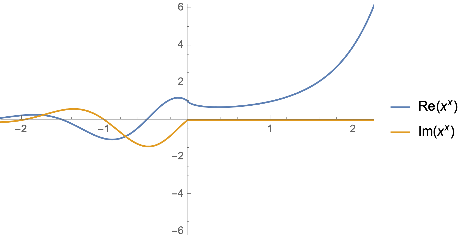
From this display, we see that the imaginary part of \( x^x \) is zero for integer values of \( x \). That’s easy enough to verify explicitly: \( (-1)^{-1} = -1, (-2)^{-2} = 1/4, (-3)^{-3} = -1/27, \cdots \).
The newest version of Mathematica has a few nice new complex number visualization options. Here’s two that I found illuminating, an absolute value plot that highlights the poles and zeros, also showing some of the phase action:
Manipulate[
ComplexPlot[ x^x, {x, s (-1 – I), s (1 + I)},
PlotLegends -> Automatic, ColorFunction -> "GlobalAbs"], {{s, 4},
0.00001, 10}]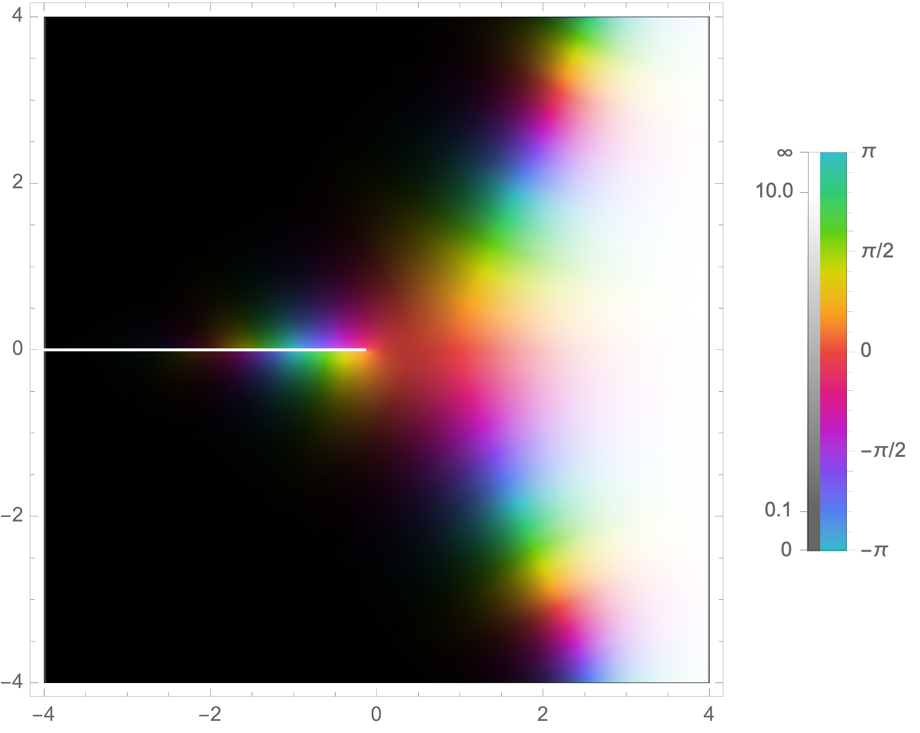
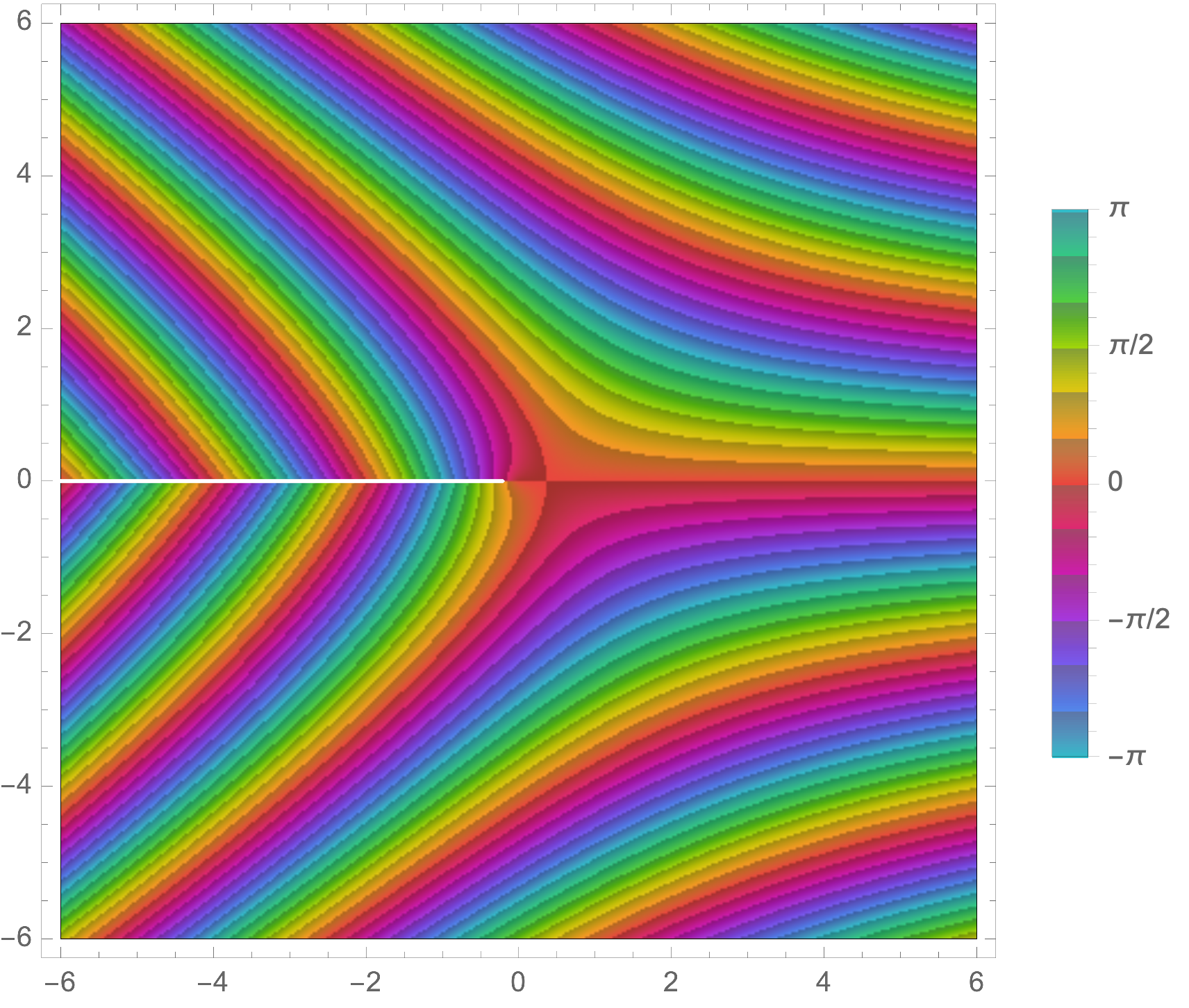
We see the branch cut nicely, the tendency to zero in the left half plane, as well as some of the phase periodicity in the regions that are in the intermediate regions between the zeros and the poles. We can also plot just the phase, which shows its interesting periodic nature
Manipulate[
ComplexPlot[ x^x, {x, s (-1 – I), s (1 + I)},
PlotLegends -> Automatic, ColorFunction -> "CyclicArg"], {{s, 6},
0.00001, 10}]
I’d like to take the time to play with some of the other ComplexPlot ColorFunction options, which appears to be a powerful and flexible visualization tool.