ece1229

Chebychev antenna array design

March 22, 2015 ece1229 , , , ,

[Click here for a PDF of this post with nicer formatting]

In our text [1] is a design procedure that applies Chebychev polynomials to the selection of current magnitudes for an evenly spaced array of identical antennas placed along the z-axis.

For an even number \( 2 M \) of identical antennas placed at positions \( \Br_m = (d/2) \lr{2 m -1} \Be_3 \), the array factor is

\begin{equation}\label{eqn:chebychevDesign:20}
\textrm{AF}
=
\sum_{m=-N}^N I_m e^{-j k \rcap \cdot \Br_m }.
\end{equation}

Assuming the currents are symmetric \( I_{-m} = I_m \), with \( \rcap = (\sin\theta \cos\phi, \sin\theta \sin\phi, \cos\theta ) \), and \( u = \frac{\pi d}{\lambda} \cos\theta \), this is

\begin{equation}\label{eqn:chebychevDesign:40}
\begin{aligned}
\textrm{AF}
&=
\sum_{m=-N}^N I_m e^{-j k (d/2) ( 2 m -1 )\cos\theta } \\
&=
2 \sum_{m=1}^N I_m \cos\lr{ k (d/2) ( 2 m -1)\cos\theta } \\
&=
2 \sum_{m=1}^N I_m \cos\lr{ (2 m -1) u }.
\end{aligned}
\end{equation}

This is a sum of only odd cosines, and can be expanded as a sum that includes all the odd powers of \( \cos u \). Suppose for example that this is a four element array with \( N = 2 \). In this case the array factor has the form

\begin{equation}\label{eqn:chebychevDesign:60}
\begin{aligned}
\textrm{AF}
&=
2 \lr{ I_1 \cos u + I_2 \lr{ 4 \cos^3 u – 3 \cos u } } \\
&=
2 \lr{ \lr{ I_1 – 3 I_2 } \cos u + 4 I_2 \cos^3 u }.
\end{aligned}
\end{equation}

The design procedure in the text sets \( \cos u = z/z_0 \), and then equates this to \( T_3(z) = 4 z^3 – 3 z \) to determine the current amplitudes \( I_m \). That is

\begin{equation}\label{eqn:chebychevDesign:80}
\frac{ 2 I_1 – 6 I_2 }{z_0} z + \frac{8 I_2}{z_0^3} z^3 = -3 z + 4 z^3,
\end{equation}

or

\begin{equation}\label{eqn:chebychevDesign:100}
\begin{aligned}
\begin{bmatrix}
I_1 \\
I_2
\end{bmatrix}
&=
{\begin{bmatrix}
2/z_0 & -6/z_0 \\
0 & 8/z_0^3
\end{bmatrix}}^{-1}
\begin{bmatrix}
-3 \\
4
\end{bmatrix} \\
&=
\frac{z_0}{2}
\begin{bmatrix}
3 (z_0^2 -1) \\
z_0^2
\end{bmatrix}.
\end{aligned}
\end{equation}

The currents in the array factor are fully determined up to a scale factor, reducing the array factor to

\begin{equation}\label{eqn:chebychevDesign:140}
\textrm{AF} = 4 z_0^3 \cos^3 u – 3 z_0 \cos u.
\end{equation}

The zeros of this array factor are located at the zeros of

\begin{equation}\label{eqn:chebychevDesign:120}
T_3( z_0 \cos u ) = \cos( 3 \cos^{-1} \lr{ z_0 \cos u } ),
\end{equation}

which are at \( 3 \cos^{-1} \lr{ z_0 \cos u } = \pi/2 + m \pi = \pi \lr{ m + \inv{2} } \)

\begin{equation}\label{eqn:chebychevDesign:160}
\cos u = \inv{z_0} \cos\lr{ \frac{\pi}{3} \lr{ m + \inv{2} } } = \setlr{ 0, \pm \frac{\sqrt{3}}{2 z_0} }.
\end{equation}

showing that the scaling factor \( z_0 \) effects the locations of the zeros. It also allows the values at the extremes \( \cos u = \pm 1 \), to increase past the \( \pm 1 \) non-scaled limit values. These effects can be explored in this Mathematica notebook, but can also be seen in fig. 1.

ChebyChevThreeScaledFig2pn

fig 1. T_3( z_0 x) for a few different scale factors z_0.


The scale factor can be fixed for a desired maximum power gain. For \( R
\textrm{dB} \), that will be when

\begin{equation}\label{eqn:chebychevDesign:180}
20 \log_{10} \cosh( 3 \cosh^{-1} z_0 ) = R \textrm{dB},
\end{equation}

or

\begin{equation}\label{eqn:chebychevDesign:200}
z_0 = \cosh \lr{ \inv{3} \cosh^{-1} \lr{ 10^{\frac{R}{20}} } }.
\end{equation}

For \( R = 30 \) dB (say), we have \( z_0 = 2.1 \), and

\begin{equation}\label{eqn:chebychevDesign:220}
\textrm{AF}
= 40 \cos^3 \lr{ \frac{\pi d}{\lambda} \cos\theta } – 6.4 \cos \lr{ \frac{\pi d}{\lambda} \cos\theta }.
\end{equation}

These are plotted in fig. 2 (linear scale), and fig. 3 (dB scale) for a couple values of \( d/\lambda \).

ChebychevT3FittingFig3pn

fig 2. T_3 fitting of 4 element array (linear scale).

ChebychevT3FittingDbFig4pn

fig 3. T_3 fitting of 4 element array (dB scale).

To explore the \( d/\lambda \) dependence try this Mathematica notebook.

References

[1] Constantine A Balanis. Antenna theory: analysis and design. John
Wiley & Sons, 3rd edition, 2005.

Updated notes for ece1229 antenna theory

March 16, 2015 ece1229 , , , , , , , , , , , , , , , , , , , , , , , , , , , , , , , , , , , , , , , , , , , , , , , , , , , , , , , , , , , , , , , , , , , , , , , , , , , , , , , , , , , , , , , , , , , , , , , , , , , , , , , , , , , , , , , , , , , , , , , , , , , , , , , , , , , , , , , , , , , , , , , , , , , , ,

I’ve now posted a first update of my notes for the antenna theory course that I am taking this term at UofT.

Unlike most of the other classes I have taken, I am not attempting to take comprehensive notes for this class. The class is taught on slides which go by faster than I can easily take notes for (and some of which match the textbook closely). In class I have annotated my copy of textbook with little details instead. This set of notes contains musings of details that were unclear, or in some cases, details that were provided in class, but are not in the text (and too long to pencil into my book), as well as some notes Geometric Algebra formalism for Maxwell’s equations with magnetic sources (something I’ve encountered for the first time in any real detail in this class).

The notes compilation linked above includes all of the following separate notes, some of which have been posted separately on this blog:

Image theorem

March 14, 2015 ece1229 , , , , , , , ,

[Click here for a PDF of this post with nicer formatting]

In the last problem set we examined the array factor for a corner cube configuration, shown in fig. 1.


homework3Fig1

fig. 1. A corner-cube antenna.


Motivation

This is a horizontal dipole antenna placed next to a metallic corner. The radiation at points in the interior of the cube have contributions due to the line of sight field from the antenna as well as reflections. We looked at an approximation of ground reflections using the \underlineAndIndex{Image Theorem}, modeling the ground as a perfectly conducting surface. I completely misunderstood that theorem and how it should be applied. As presented it seemed like a simple way to figure out the reflection characteristics. This confused me since it did not seem consistent with Fresnel reflection theory. I did try to reconcile to the two, but that reconciliation only appeared to work for certain dipole orientations, and that orientation dependence remained an open question.

It turns out that the idea of the Image Theorem is to find a source configuration that contains the specified source, but contains enough other sources that the tangential component of the electric field superposition is zero on the conducting surface, as required by Maxwell’s equations. This allows the boundary to be completely removed from the problem.

Thinking of the corner cube configuration as a reflection problem, I positioned sources as in fig. 2.


incorrectImagePlacementForCornerCubeFig2

fig. 2. Incorrect Image Theorem source placement for corner cube.


Because of the horizontal orientation of the dipole, I argued that the reflection coefficient should be -1. The reflection point is a bit messy to calculate, and it turns out to zeroth order in \( h/r \) the \( \sin\theta \) magnitude scaling of the reflected (far-field) field is present for both reflected rays. I though that this was probably because the observation point lays at the same altitude for both the line of sight ray and the reflected ray.

Attempting this problem as a reflection problem makes it much more difficult than it needs to be. It turns out that the correct image source placement for this problem is that of fig. 3.


cornerCubeImageSourcePlacementFig3

fig. 3. Correct image source placement for the corner cube.


This wasn’t at all obvious to me. The key is understanding that the goal of the image source placement isn’t to figure out how the reflection will occur, but to manufacture a source configuration for which the tangential component of the electric field is zero on the conducting surface.

Image placement for infinite conducting plane.

Before thinking about the corner cube configuration, consider a horizontal dipole next to an infinite conducting plane. This, and the correct image source placement is illustrated in fig. 4.


reflectionOfImagePointsFig1

fig. 4. Image source placement for horizontal dipole.


I’ll now verify that this is the correct image source. This is basically a calculation that the tangential components of the electric fields from both sources sum to zero.

Let,

\begin{equation}\label{eqn:imageTheorem:20}
r = \Abs{\Bs – \Br_0},
\end{equation}

so that the magnetic vector potential for the first quadrant dipole has the form

\begin{equation}\label{eqn:imageTheorem:40}
\BA = \frac{A_0}{4 \pi r} e^{-j k r} \zcap.
\end{equation}

With

\begin{equation}\label{eqn:imageTheorem:60}
\begin{aligned}
\kcap &= \frac{\Bs – \Br_0}{s} \\
\tilde{\BE} &= \zcap – \lr{\zcap \cdot \kcap} \kcap,
\end{aligned}
\end{equation}

the far-field electric field at the point \( \Bs \) on the plane is

\begin{equation}\label{eqn:imageTheorem:80}
\BE = -j \omega \frac{A_0}{4 \pi r} e^{-j k r} \tilde{\BE}.
\end{equation}

If the normal to the plane is \( \ncap \) the tangential component of this field is the projection of \( \BE \) on the direction

\begin{equation}\label{eqn:imageTheorem:100}
\pcap = \frac{\kcap \cross \ncap}{\Abs{\kcap \cross \ncap}}.
\end{equation}

That tangential component is directed along

\begin{equation}\label{eqn:imageTheorem:120}
\lr{\tilde{\BE} \cdot \pcap } \pcap
=
\lr{\lr{\zcap – \lr{\zcap \cdot \kcap} \kcap} \cdot \lr{\kcap \cross \ncap}} \frac{\kcap \cross \ncap}{\Abs{\kcap \cross \ncap}^2}.
\end{equation}

Because the triple product \( \kcap \cdot \lr{\kcap \cross \ncap} = 0 \), the tangential component of the electric field, provided \( \kcap \cdot \ncap \ne 0 \), is

\begin{equation}\label{eqn:imageTheorem:140}
\BE_\parallel
=
-j \omega \frac{A_0}{4 \pi r} e^{-j k r} \zcap \cdot \lr{\kcap \cross \ncap} \frac{\kcap \cross \ncap}{ 1 – \lr{ \ncap \cdot \kcap }^2 }.
\end{equation}

Now the wave vector direction for the second quadrant ray on the plane is required. Both \( \kcap’ \) and \( \Bs’ \) are reflections across the plane. Any such reflection has the value

\begin{equation}\label{eqn:imageTheorem:160}
\begin{aligned}
\Bx’
&= \lr{ \Bx \wedge \ncap} \ncap – \lr{ \Bx \cdot \ncap } \ncap \\
&= – \lr{ \ncap \wedge \Bx + \ncap \cdot \Bx } \ncap \\
&= – \ncap \Bx \ncap.
\end{aligned}
\end{equation}

This multivector product nicely encapsulates the reflection operation. Consider a reflection against the y-z plane with normal \( \Be_1 \) to verify that this works

\begin{equation}\label{eqn:imageTheorem:180}
\begin{aligned}
-\Be_1 \Bx \Be_1
&=
-\Be_1 \lr{ x \Be_1 + y \Be_2 + z \Be_3 } \Be_1 \\
&=
-\lr{ x – y \Be_2 \Be_1 + z \Be_3 \Be_1 } \Be_1 \\
&=
-\lr{ x \Be_1 – y \Be_2 + z \Be_3 } \\
&=
– x \Be_1 + y \Be_2 + z \Be_3.
\end{aligned}
\end{equation}

This has the x component flipped in sign and the rest left untouched as desired for a reflection in the y-z plane.

The second quadrant field will have \( \kcap’ \cross \ncap \) terms in place of all the \( \kcap \cross \ncap \) terms of \ref{eqn:imageTheorem:140}. We want to know how the two compare. This calculation is simply done using the dual form of the cross product temporarily

\begin{equation}\label{eqn:imageTheorem:200}
\begin{aligned}
\kcap’ \cross \ncap
&=
-I \lr{ \kcap’ \wedge \ncap} \\
&=
-I \gpgradetwo{\kcap’ \ncap} \\
&=
-I \gpgradetwo{ {-\ncap \kcap \ncap} \ncap} \\
&=
I \gpgradetwo{ \ncap \kcap } \\
&=
I \ncap \wedge \kcap \\
&=
-\ncap \cross \kcap \\
&=
\kcap \cross \ncap.
\end{aligned}
\end{equation}

So, provided the image source in the second quadrant is oppositely oriented (sign inversion), the tangential components of the two will sum to zero on that surface.

Thinking back to the corner cube, it is clear that an image source opposite to the source across from one of the walls will result in a zero tangential electric field along this boundary as is the case here (say the y-z plane). A second pair of sources opposite from each other anywhere else also about the y-z plane will not change that zero tangential electric field on this surface, but if the signs of the sources is alternated as in fig. 3 it will also result in zero tangential electric field on the z-x plane, which has the desired boundary value effects for both surfaces of the corner cube.

Tschebyscheff polynomials

March 13, 2015 ece1229 , , ,

[Click here for a PDF of this post with nicer formatting]

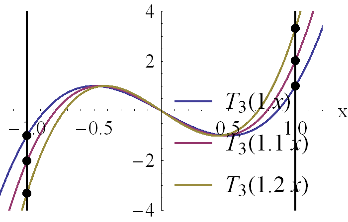
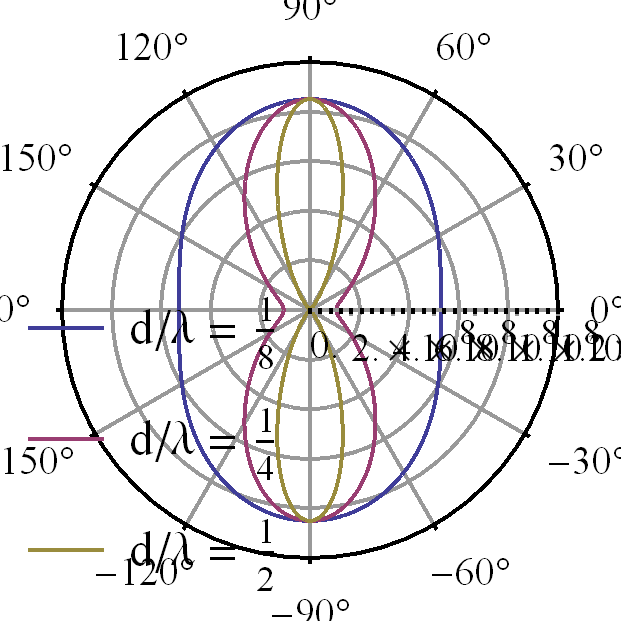
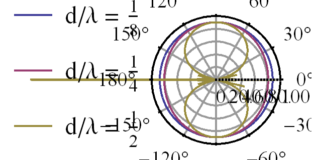
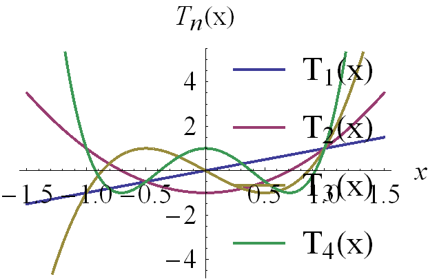
In ancient times (i.e. 2nd year undergrad) I recall being very impressed with Tschebyscheff polynomials for designing lowpass filters. I’d used Tschebyscheff filters for the hardware we used for a speech recognition system our group built in the design lab. One of the benefits of these polynomials is that the oscillation in the \( \Abs{x} < 1 \) interval is strictly bounded. This same property, as well as the unbounded nature outside of the \( [-1,1] \) interval turns out to have applications to antenna array design.

The Tschebyscheff polynomials are defined by

\begin{equation}\label{eqn:tschebyscheff:40}
T_m(x) = \cos\lr{ m \cos^{-1} x }, \quad \Abs{x} < 1 \end{equation} \begin{equation}\label{eqn:tschebyscheff:60} T_m(x) = \cosh\lr{ m \cosh^{-1} x }, \quad \Abs{x} > 1.
\end{equation}

Range restrictions and hyperbolic form.

Prof. Eleftheriades’s notes made a point to point out the definition in the \( \Abs{x} > 1 \) interval, but that can also be viewed as a consequence instead of a definition if the range restriction is removed. For example, suppose \( x = 7 \), and let

\begin{equation}\label{eqn:tschebyscheff:160}
\cos^{-1} 7 = \theta,
\end{equation}

so
\begin{equation}\label{eqn:tschebyscheff:180}
\begin{aligned}
7
&= \cos\theta \\
&= \frac{e^{i\theta} + e^{-i\theta}}{2} \\
&= \cosh(i\theta),
\end{aligned}
\end{equation}

or

\begin{equation}\label{eqn:tschebyscheff:200}
-i \cosh^{-1} 7 = \theta.
\end{equation}

\begin{equation}\label{eqn:tschebyscheff:220}
\begin{aligned}
T_m(7)
&= \cos( -m i \cosh^{-1} 7 ) \\
&= \cosh( m \cosh^{-1} 7 ).
\end{aligned}
\end{equation}

The same argument clearly applies to any other value outside of the \( \Abs{x} < 1 \) range, so without any restrictions, these polynomials can be defined as just

\begin{equation}\label{eqn:tschebyscheff:260}
\boxed{
T_m(x) = \cos\lr{ m \cos^{-1} x }.
}
\end{equation}

Polynomial nature.

Eq. \ref{eqn:tschebyscheff:260} does not obviously look like a polynomial. Let’s proceed to verify the polynomial nature for the first couple values of \( m \).

  • \( m = 0 \).\begin{equation}\label{eqn:tschebyscheff:280}
    \begin{aligned}
    T_0(x)
    &= \cos( 0 \cos^{-1} x ) \\
    &= \cos( 0 ) \\
    &= 1.
    \end{aligned}
    \end{equation}
  • \( m = 1 \).\begin{equation}\label{eqn:tschebyscheff:300}
    \begin{aligned}
    T_1(x)
    &= \cos( 1 \cos^{-1} x ) \\
    &= x.
    \end{aligned}
    \end{equation}
  • \( m = 2 \).\begin{equation}\label{eqn:tschebyscheff:320}
    \begin{aligned}
    T_2(x)
    &= \cos( 2 \cos^{-1} x ) \\
    &= 2 \cos^2 \cos^{-1}(x) – 1 \\
    &= 2 x^2 – 1.
    \end{aligned}
    \end{equation}

To examine the general case

\begin{equation}\label{eqn:tschebyscheff:340}
\begin{aligned}
T_m(x)
&= \cos( m \cos^{-1} x ) \\
&= \textrm{Re} e^{ j m \cos^{-1} x } \\
&= \textrm{Re} \lr{ e^{ j\cos^{-1} x } }^m \\
&= \textrm{Re} \lr{ \cos\cos^{-1} x + j \sin\cos^{-1} x }^m \\
&= \textrm{Re} \lr{ x + j \sqrt{1 – x^2} }^m \\
&=
\textrm{Re} \lr{
x^m
+ \binom{ m}{1} j x^{m-1} \lr{1 – x^2}^{1/2}
– \binom{ m}{2} x^{m-2} \lr{1 – x^2}^{2/2}
– \binom{ m}{3} j x^{m-3} \lr{1 – x^2}^{3/2}
+ \binom{ m}{4} x^{m-4} \lr{1 – x^2}^{4/2}
+ \cdots
} \\
&=
x^m
– \binom{ m}{2} x^{m-2} \lr{1 – x^2}
+ \binom{ m}{4} x^{m-4} \lr{1 – x^2}^2
– \cdots
\end{aligned}
\end{equation}

This expansion was a bit cavaliar with the signs of the \( \sin\cos^{-1} x = \sqrt{1 – x^2} \) terms, since the negative sign should be picked for the root when \( x \in [-1,0] \). However, that doesn’t matter in the end since the real part operation selects only powers of two of this root.

The final result of the expansion above can be written

\begin{equation}\label{eqn:tschebyscheff:360}
\boxed{
T_m(x) = \sum_{k = 0}^{\lfloor m/2 \rfloor} \binom{m}{2 k} (-1)^k x^{m – 2 k} \lr{1 – x^2}^k.
}
\end{equation}

This clearly shows the polynomial nature of these functions, and is also perfectly well defined for any value of \( x \). The even and odd alternation with \( m \) is also clear in this explicit expansion.
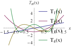
Plots

ChebychevFig1pn

Properties

In [1] a few properties can be found for these polynomials

\begin{equation}\label{eqn:tschebyscheff:100}
T_m(x) = 2 x T_{m-1} – T_{m-2}
\end{equation}
\begin{equation}\label{eqn:tschebyscheff:420}
0 = \lr{ 1 – x^2 } \frac{d T_m(x)}{dx} + m x T_m(x) – m T_{m-1}(x)
\end{equation}
\begin{equation}\label{eqn:tschebyscheff:400}
0 = \lr{ 1 – x^2 } \frac{d^2 T_m(x)}{dx^2} – x \frac{dT_m(x)}{dx} + m^2 T_{m}(x)
\end{equation}
\begin{equation}\label{eqn:tschebyscheff:440}
\int_{-1}^1 \inv{ \sqrt{1 – x^2} } T_m(x) T_n(x) dx =
\left\{
\begin{array}{l l}
0 & \quad \mbox{if \( m \ne n \) } \\
\pi & \quad \mbox{if \( m = n = 0 \) } \\
\pi/2 & \quad \mbox{if \( m = n, m \ne 0 \) }
\end{array}
\right.
\end{equation}

Recurrance relation.

Prove \ref{eqn:tschebyscheff:100}.

Answer.

To show this, let

\begin{equation}\label{eqn:tschebyscheff:460}
x = \cos\theta.
\end{equation}

\begin{equation}\label{eqn:tschebyscheff:580}
2 x T_{m-1} – T_{m-2}
=
2 \cos\theta \cos((m-1) \theta) – \cos((m-2)\theta).
\end{equation}

Recall the cosine addition formulas

\begin{equation}\label{eqn:tschebyscheff:540}
\begin{aligned}
\cos( a + b )
&=
\textrm{Re} e^{j(a + b)} \\
&=
\textrm{Re} e^{ja} e^{jb} \\
&=
\textrm{Re}
\lr{ \cos a + j \sin a }
\lr{ \cos b + j \sin b } \\
&=
\cos a \cos b – \sin a \sin b.
\end{aligned}
\end{equation}

Applying this gives

\begin{equation}\label{eqn:tschebyscheff:600}
\begin{aligned}
2 x T_{m-1} – T_{m-2}
&=
2 \cos\theta \Biglr{ \cos(m\theta)\cos\theta +\sin(m\theta) \sin\theta }
– \Biglr{
\cos(m\theta)\cos(2\theta) + \sin(m\theta) \sin(2\theta)
} \\
&=
2 \cos\theta \Biglr{ \cos(m\theta)\cos\theta +\sin(m\theta)\sin\theta) }
– \Biglr{
\cos(m\theta)(\cos^2 \theta – \sin^2 \theta) + 2 \sin(m\theta) \sin\theta \cos\theta
} \\
&=
\cos(m\theta) \lr{ \cos^2\theta + \sin^2\theta } \\
&= T_m(x).
\end{aligned}
\end{equation}

First order LDE relation.

Prove \ref{eqn:tschebyscheff:420}.

Answer.

To show this, again, let

\begin{equation}\label{eqn:tschebyscheff:470}
x = \cos\theta.
\end{equation}

Observe that

\begin{equation}\label{eqn:tschebyscheff:480}
1 = -\sin\theta \frac{d\theta}{dx},
\end{equation}

so

\begin{equation}\label{eqn:tschebyscheff:500}
\begin{aligned}
\frac{d}{dx}
&= \frac{d\theta}{dx} \frac{d}{d\theta} \\
&= -\frac{1}{\sin\theta} \frac{d}{d\theta}.
\end{aligned}
\end{equation}

Plugging this in gives

\begin{equation}\label{eqn:tschebyscheff:520}
\begin{aligned}
\lr{ 1 – x^2} &\frac{d}{dx} T_m(x) + m x T_m(x) – m T_{m-1}(x) \\
&=
\sin^2\theta
\lr{
-\frac{1}{\sin\theta} \frac{d}{d\theta}}
\cos( m \theta ) + m \cos\theta \cos( m \theta ) – m \cos( (m-1)\theta ) \\
&=
-\sin\theta (-m \sin(m \theta)) + m \cos\theta \cos( m \theta ) – m \cos( (m-1)\theta ).
\end{aligned}
\end{equation}

Applying the cosine addition formula \ref{eqn:tschebyscheff:540} gives

\begin{equation}\label{eqn:tschebyscheff:560}
m \lr{ \sin\theta \sin(m \theta) + \cos\theta \cos( m \theta ) } – m
\lr{
\cos( m \theta) \cos\theta + \sin( m \theta ) \sin\theta
}
=0.
\end{equation}

} % answer

Second order LDE relation.

Prove \ref{eqn:tschebyscheff:400}.

Answer.

This follows the same way. The first derivative was

\begin{equation}\label{eqn:tschebyscheff:640}
\begin{aligned}
\frac{d T_m(x)}{dx}
&=
-\inv{\sin\theta}
\frac{d}{d\theta} \cos(m\theta) \\
&=
-\inv{\sin\theta} (-m) \sin(m\theta) \\
&=
m \inv{\sin\theta} \sin(m\theta),
\end{aligned}
\end{equation}

so the second derivative is

\begin{equation}\label{eqn:tschebyscheff:620}
\begin{aligned}
\frac{d^2 T_m(x)}{dx^2}
&=
-m \inv{\sin\theta} \frac{d}{d\theta} \inv{\sin\theta} \sin(m\theta) \\
&=
-m \inv{\sin\theta}
\lr{
-\frac{\cos\theta}{\sin^2\theta} \sin(m\theta) + \inv{\sin\theta} m \cos(m\theta)
}.
\end{aligned}
\end{equation}

Putting all the pieces together gives

\begin{equation}\label{eqn:tschebyscheff:660}
\begin{aligned}
\lr{ 1 – x^2 } &\frac{d^2 T_m(x)}{dx^2} – x \frac{dT_m(x)}{dx} + m^2 T_{m}(x) \\
&=
m
\lr{
\frac{\cos\theta}{\sin\theta} \sin(m\theta) – m \cos(m\theta)
}
– \cos\theta m \inv{\sin\theta} \sin(m\theta)
+ m^2 \cos(m \theta) \\
&=
0.
\end{aligned}
\end{equation}

Orthogonality relation

Prove \ref{eqn:tschebyscheff:440}.

Answer.

First consider the 0,0 inner product, making an \( x = \cos\theta \), so that \( dx = -\sin\theta d\theta \)

\begin{equation}\label{eqn:tschebyscheff:680}
\begin{aligned}
\innerprod{T_0}{T_0}
&=
\int_{-1}^1 \inv{\lr{1-x^2}^{1/2}} dx \\
&=
\int_{-\pi}^0 \lr{-\inv{\sin\theta}} -\sin\theta d\theta \\
&=
0 – (-\pi) \\
&= \pi.
\end{aligned}
\end{equation}

Note that since the \( [-\pi, 0] \) interval was chosen, the negative root of \( \sin^2\theta = 1 – x^2 \) was chosen, since \( \sin\theta \) is negative in that interval.

The m,m inner product with \( m \ne 0 \) is

\begin{equation}\label{eqn:tschebyscheff:700}
\begin{aligned}
\innerprod{T_m}{T_m}
&=
\int_{-1}^1 \inv{\lr{1-x^2}^{1/2}} \lr{ T_m(x)}^2 dx \\
&=
\int_{-\pi}^0 \lr{-\inv{\sin\theta}} \cos^2(m\theta) -\sin\theta d\theta \\
&=
\int_{-\pi}^0 \cos^2(m\theta) d\theta \\
&=
\inv{2} \int_{-\pi}^0 \lr{ \cos(2 m\theta) + 1 } d\theta \\
&= \frac{\pi}{2}.
\end{aligned}
\end{equation}

So far so good. For \( m \ne n \) the inner product is

\begin{equation}\label{eqn:tschebyscheff:720}
\begin{aligned}
\innerprod{T_m}{T_m}
&=
\int_{-\pi}^0 \cos(m\theta) \cos(n\theta) d\theta \\
&=
\inv{4} \int_{-\pi}^0
\lr{
e^{j m \theta}
+ e^{-j m \theta}
}
\lr{
e^{j n \theta}
+ e^{-j n \theta}
}
d\theta \\
&=
\inv{4} \int_{-\pi}^0
\lr{
e^{j (m + n) \theta}
+e^{-j (m + n) \theta}
+e^{j (m – n) \theta}
+e^{j (-m + n) \theta}
}
d\theta \\
&=
\inv{2} \int_{-\pi}^0
\lr{
\cos( (m + n)\theta )
+\cos( (m – n)\theta )
}
d\theta \\
&=
\inv{2}
\evalrange{
\lr{
\frac{\sin( (m + n)\theta )}{ m + n }
+\frac{\sin( (m – n)\theta )}{ m – n}
}
}{-\pi}{0} \\
&= 0.
\end{aligned}
\end{equation}

References

[1] M. Abramowitz and I.A. Stegun. Handbook of mathematical functions with formulas, graphs, and mathematical tables, volume 55. Dover publications, 1964.

Parallel projection of electromagnetic fields with Geometric Algebra

March 8, 2015 ece1229 , , , ,

[Click here for a PDF of this post with nicer formatting]

When computing the components of a polarized reflecting ray that were parallel or not-parallel to the reflecting surface, it was found that the electric and magnetic fields could be written as

\begin{equation}\label{eqn:gaFieldProjection:280}
\BE = \lr{ \BE \cdot \pcap } \pcap + \lr{ \BE \cdot \qcap } \qcap = E_\parallel \pcap + E_\perp \qcap
\end{equation}
\begin{equation}\label{eqn:gaFieldProjection:300}
\BH = \lr{ \BH \cdot \pcap } \pcap + \lr{ \BH \cdot \qcap } \qcap = H_\parallel \pcap + H_\perp \qcap.
\end{equation}

where a unit vector \( \pcap \) that lies both in the reflecting plane and in the electromagnetic plane (tangential to the wave vector direction) was

\begin{equation}\label{eqn:gaFieldProjection:340}
\pcap = \frac{\kcap \cross \ncap}{\Abs{\kcap \cross \ncap}}
\end{equation}
\begin{equation}\label{eqn:gaFieldProjection:360}
\qcap = \kcap \cross \pcap.
\end{equation}

Here \( \qcap \) is perpendicular to \( \pcap \) but lies in the electromagnetic plane. This logically subdivides the fields into two pairs, one with the electric field parallel to the reflection plane

\begin{equation}\label{eqn:gaFieldProjection:240}
\begin{aligned}
\BE_1 &= \lr{ \BE \cdot \pcap } \pcap = E_\parallel \pcap \\
\BH_1 &= \lr{ \BH \cdot \qcap } \qcap = H_\perp \qcap,
\end{aligned}
\end{equation}

and one with the magnetic field parallel to the reflection plane

\begin{equation}\label{eqn:gaFieldProjection:380}
\begin{aligned}
\BH_2 &= \lr{ \BH \cdot \pcap } \pcap = H_\parallel \pcap \\
\BE_2 &= \lr{ \BE \cdot \qcap } \qcap = E_\perp \qcap.
\end{aligned}
\end{equation}

Expressed in Geometric Algebra form, each of these pairs of fields should be thought of as components of a single multivector field. That is

\begin{equation}\label{eqn:gaFieldProjection:400}
F_1 = \BE_1 + c \mu_0 \BH_1 I
\end{equation}
\begin{equation}\label{eqn:gaFieldProjection:460}
F_2 = \BE_2 + c \mu_0 \BH_2 I
\end{equation}

where the original total field is

\begin{equation}\label{eqn:gaFieldProjection:420}
F = \BE + c \mu_0 \BH I.
\end{equation}

In \ref{eqn:gaFieldProjection:400} we have a composite projection operation, finding the portion of the electric field that lies in the reflection plane, and simultaneously finding the component of the magnetic field that lies perpendicular to that (while still lying in the tangential plane of the electromagnetic field). In \ref{eqn:gaFieldProjection:460} the magnetic field is projected onto the reflection plane and a component of the electric field that lies in the tangential (to the wave vector direction) plane is computed.

If we operate only on the complete multivector field, can we find these composite projection field components in a single operation, instead of working with the individual electric and magnetic fields?

Working towards this goal, it is worthwhile to point out consequences of the assumption that the fields are plane wave (or equivalently far field spherical waves). For such a wave we have

\begin{equation}\label{eqn:gaFieldProjection:480}
\begin{aligned}
\BH
&= \inv{\mu_0} \kcap \cross \BE \\
&= \inv{\mu_0} (-I)\lr{ \kcap \wedge \BE } \\
&= \inv{\mu_0} (-I)\lr{ \kcap \BE – \kcap \cdot \BE} \\
&= -\frac{I}{\mu_0} \kcap \BE,
\end{aligned}
\end{equation}

or

\begin{equation}\label{eqn:gaFieldProjection:520}
\mu_0 \BH I = \kcap \BE.
\end{equation}

This made use of the identity \( \Ba \wedge \Bb = I \lr{\Ba \cross \Bb} \), and the fact that the electric field is perpendicular to the wave vector direction. The total multivector field is

\begin{equation}\label{eqn:gaFieldProjection:500}
\begin{aligned}
F
&= \BE + c \mu_0 \BH I \\
&= \lr{ 1 + c \kcap } \BE.
\end{aligned}
\end{equation}

Expansion of magnetic field component that is perpendicular to the reflection plane gives

\begin{equation}\label{eqn:gaFieldProjection:540}
\begin{aligned}
\mu_0 H_\perp
&= \mu_0 \BH \cdot \qcap \\
&= \gpgradezero{ \lr{-\kcap \BE I} \qcap } \\
&= -\gpgradezero{ \kcap \BE I \lr{ \kcap \cross \pcap} } \\
&= \gpgradezero{ \kcap \BE I I \lr{ \kcap \wedge \pcap} } \\
&= -\gpgradezero{ \kcap \BE \kcap \pcap } \\
&= \gpgradezero{ \kcap \kcap \BE \pcap } \\
&= \BE \cdot \pcap,
\end{aligned}
\end{equation}

so

\begin{equation}\label{eqn:gaFieldProjection:560}
F_1
= (\pcap + c I \qcap ) \BE \cdot \pcap.
\end{equation}

Since \( \qcap \kcap \pcap = I \), the component of the complete multivector field in the \( \pcap \) direction is

\begin{equation}\label{eqn:gaFieldProjection:580}
\begin{aligned}
F_1
&= (\pcap – c \pcap \kcap ) \BE \cdot \pcap \\
&= \pcap (1 – c \kcap ) \BE \cdot \pcap \\
&= (1 + c \kcap ) \pcap \BE \cdot \pcap.
\end{aligned}
\end{equation}

It is reasonable to expect that \( F_2 \) has a similar form, but with \( \pcap \rightarrow \qcap \). This is verified by expansion

\begin{equation}\label{eqn:gaFieldProjection:600}
\begin{aligned}
F_2
&= E_\perp \qcap + c \lr{ \mu_0 H_\parallel } \pcap I \\
&= \lr{\BE \cdot \qcap} \qcap + c \gpgradezero{ – \kcap \BE I \kcap \qcap I } \lr{\kcap \qcap I} I \\
&= \lr{\BE \cdot \qcap} \qcap + c \gpgradezero{ \kcap \BE \kcap \qcap } \kcap \qcap (-1) \\
&= \lr{\BE \cdot \qcap} \qcap + c \gpgradezero{ \kcap \BE (-\qcap \kcap) } \kcap \qcap (-1) \\
&= \lr{\BE \cdot \qcap} \qcap + c \gpgradezero{ \kcap \kcap \BE \qcap } \kcap \qcap \\
&= \lr{ 1 + c \kcap } \qcap \lr{ \BE \cdot \qcap }
\end{aligned}
\end{equation}

This and \ref{eqn:gaFieldProjection:580} before that makes a lot of sense. The original field can be written

\begin{equation}\label{eqn:gaFieldProjection:620}
F = \lr{ \Ecap + c \lr{ \kcap \cross \Ecap } I } \BE \cdot \Ecap,
\end{equation}

where the leading multivector term contains all the directional dependence of the electric and magnetic field components, and the trailing scalar has the magnitude of the field with respect to the reference direction \( \Ecap \).

We have the same structure after projecting \( \BE \) onto either the \( \pcap \), or \( \qcap \) directions respectively

\begin{equation}\label{eqn:gaFieldProjection:660}
F_1 = \lr{ \pcap + c \lr{ \kcap \cross \pcap } I} \BE \cdot \pcap
\end{equation}
\begin{equation}\label{eqn:gaFieldProjection:680}
F_2 = \lr{ \qcap + c \lr{ \kcap \cross \qcap } I} \BE \cdot \qcap.
\end{equation}

The next question is how to achieve this projection operation directly in terms of \( F \) and \( \pcap, \qcap \), without resorting to expression of \( F \) in terms of \( \BE \), and \( \BB \). I’ve not yet been able to determine the structure of that operation.