phy2403

New aggregate collection of notes for PHY2403, QFT I : up to lecture 21.

December 2, 2018 phy2403

I’ve now uploaded a new version of my class notes for PHY2403, the UofT Quantum Field Theory I course, taught this year by Prof. Erich Poppitz.

This version includes the following content.  Fermion related content is new since the last upload, as well as some work to make the scattering content (lecture 17,18) somewhat sensible (it was in it’s raw post-class form before, which made little sense)

  • Chapter 1: Fields, units, and scales.
  • 1.1: What is a field?
  • 1.2: Scales.
  • 1.3: Natural units.
  • 1.4: Gravity.
  • 1.5: Cross section.
  • 1.6: Problems.
  • Chapter 2: Lorentz transformations.
  • 2.1: Lorentz transformations.
  • 2.2: Determinant of Lorentz transformations.
  • 2.3: Problems.
  • Chapter 3: Classical field theory.
  • 3.1: Field theory.
  • 3.2: Actions.
  • 3.3: Principles determining the form of the action.
  • 3.4: Principles (cont.)
  • 3.5: Least action principle.
  • 3.6: Problems.
  • Chapter 4: Canonical quantization, Klein-Gordon equation, SHOs, momentum space representation, raising and lowering operators.
  • 4.1: Canonical quantization.
  • 4.2: Canonical quantization (cont.)
  • 4.3: Momentum space representation.
  • 4.4: Quantization of Field Theory.
  • 4.5: Free Hamiltonian.
  • 4.6: QM SHO review.
  • 4.7: Discussion.
  • 4.8: Problems.
  • Chapter 5: Symmetries.
  • 5.1: Switching gears: Symmetries.
  • 5.2: Symmetries.
  • 5.3: Spacetime translation.
  • 5.4: 1st Noether theorem.
  • 5.5: Unitary operators.
  • 5.6: Continuous symmetries.
  • 5.7: Classical scalar theory.
  • 5.8: Last time.
  • 5.9: Examples of symmetries.
  • 5.10: Scale invariance.
  • 5.11: Lorentz invariance.
  • 5.12: Problems.
  • Chapter 6: Lorentz boosts, generators, Lorentz invariance, microcausality.
  • 6.1: Lorentz transform symmetries.
  • 6.2: Transformation of momentum states.
  • 6.3: Relativistic normalization.
  • 6.4: Spacelike surfaces.
  • 6.5: Condition on microcausality.
  • Chapter 7: External sources
  • 7.1: Harmonic oscillator.
  • 7.2: Field theory (where we are going).
  • 7.3: Green’s functions for the forced Klein-Gordon equation.
  • 7.4: Pole shifting.
  • 7.5: Matrix element representation of the Wightman function.
  • 7.6: Retarded Green’s function.
  • 7.7: Review: “particle creation problem”.
  • 7.8: Digression: coherent states.
  • 7.9: Problems.
  • Chapter 8: Perturbation theory.
  • 8.1: Feynman’s Green’s function
  • 8.2: Interacting field theory: perturbation theory in QFT.
  • 8.3: Perturbation theory, interaction representation and Dyson formula
  • 8.4: Next time.
  • 8.5: Review
  • 8.6: Perturbation
  • 8.7: Review
  • 8.8: Unpacking it.
  • 8.9: Calculating perturbation
  • 8.10: Wick contractions
  • 8.11: Simplest Feynman diagrams
  • 8.12: Phi fourth interaction
  • 8.13: Tree level diagrams.
  • 8.14: Problems.
  • Chapter 9: Scattering and decay.
  • 9.1: Definitions and motivation.
  • 9.2: Definitions and motivation (cont.)
  • 9.3: Calculating interactions
  • 9.4: Example diagrams.
  • 9.5: The recipe.
  • 9.6: Back to our scalar theory
  • 9.7: Review: S-matrix
  • 9.8: Scattering in a scalar theory
  • 9.9: Decay rates.
  • 9.10: Cross section.
  • 9.11: More on cross section.
  • 9.12: d(LIPS)_2.
  • 9.13: Problems.
  • Chapter 10: Fermions, and spinors.
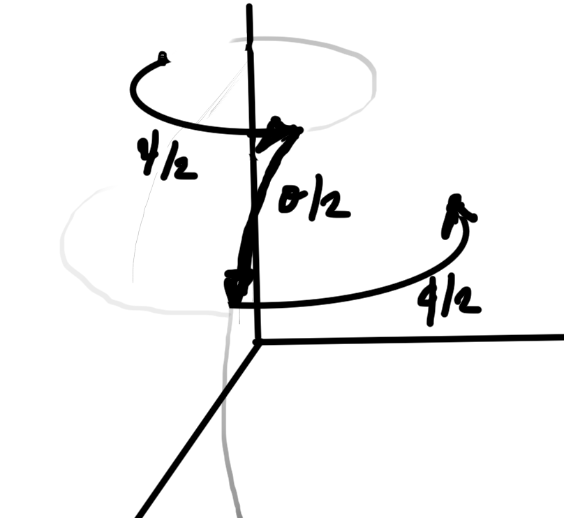
  • 10.1: Fermions: R3 rotations.
  • 10.2: Lorentz group
  • 10.3: Weyl spinors.
  • 10.4: Lorentz symmetry.
  • 10.5: Dirac matrices.
  • 10.6: Dirac Lagrangian.
  • 10.7: Review.
  • 10.8: Dirac equation.
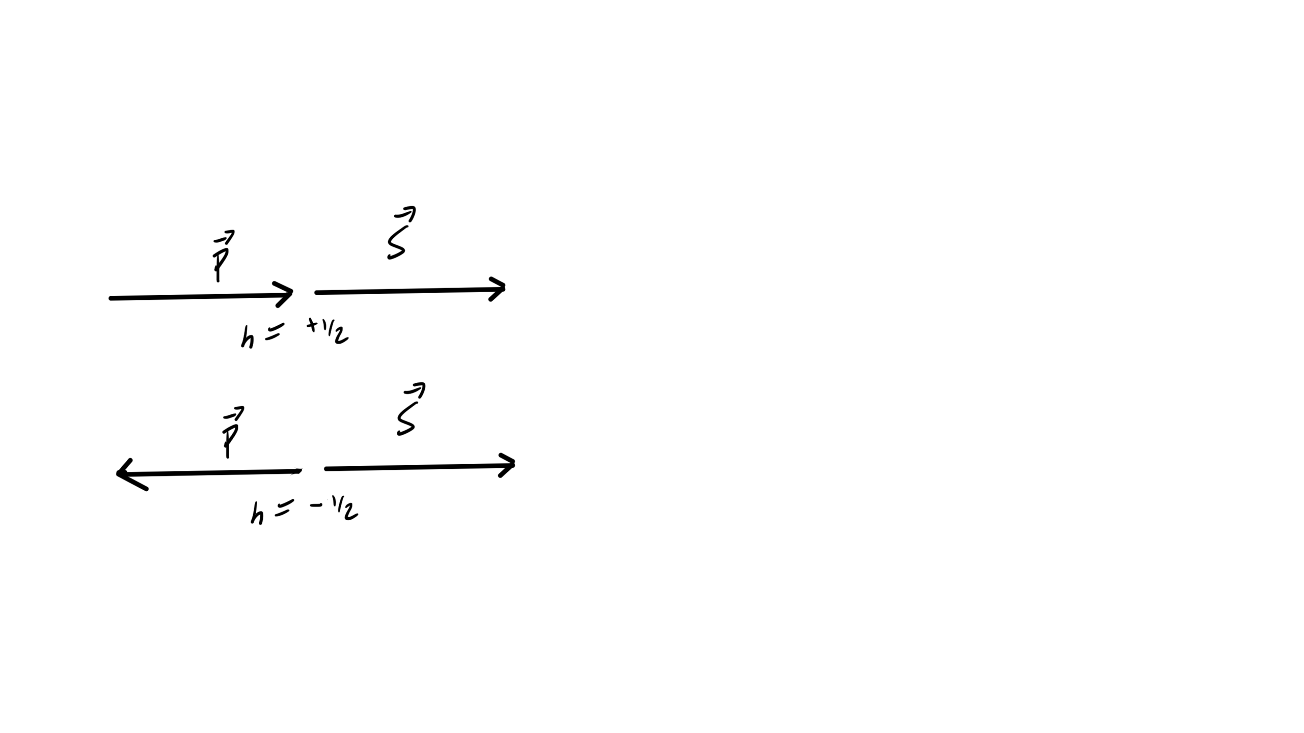
  • 10.9: Helicity
  • 10.10: Next time.
  • 10.11: Review.
  • 10.12: Normalization.
  • 10.13: Other solution.
  • 10.14: Lagrangian.
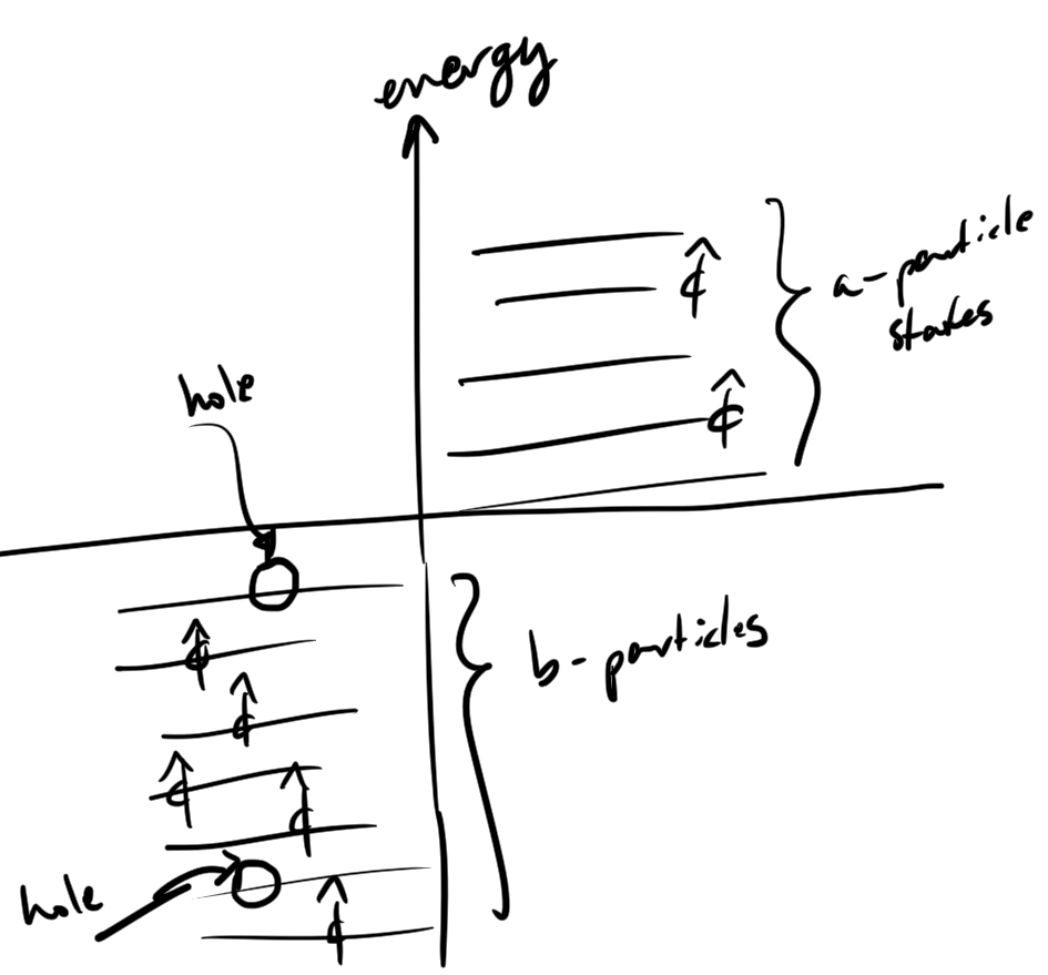
  • 10.15: General solution and Hamiltonian.
  • 10.16: Problems.
  • Appendix A: A Useful formulas and review.
  • A.1: Review of old material.
  • A.2: Useful results from new material.
  • Appendix B: Momentum of scalar field.
  • B.1: Expansion of the field momentum.
  • B.2: Conservation of the field momentum.
  • Appendix C: Reflection using Pauli matrices.

Problem set 1-3 solutions are redacted.  If interested (and not a future student of PHY2403), feel free to contact me for an un-redacted copy.

PHY2403H Quantum Field Theory. Lecture 21, Part II: Dirac Hamiltonian, Hamiltonian eigenvalues, general solution, creation and anhillation operators, Dirac Sea, antielectrons. Taught by Prof. Erich Poppitz

December 1, 2018 phy2403 , , , , ,

This post contains a summary of my lecture notes for the second half of last Wednesday’s QFT-I lecture.
[Click here for a PDF with the full notes for this portion of the lecture.]

DISCLAIMER: Very rough notes from class, with some additional side notes.

These are notes for the UofT course PHY2403H, Quantum Field Theory, taught by Prof. Erich Poppitz, fall 2018.

Summary:

  • We found that the Dirac Hamiltonian is
    \begin{equation*}
    H
    =
    \int d^3 x
    \Psi^\dagger
    \lr{
    – i \gamma^0 \gamma^j \partial_j \Psi + m \gamma^0
    }
    \Psi.
    \end{equation*}
  • We found that our plane wave solutions
    \(\Psi_u = u(p) e^{-i p \cdot x}\), and \( \Psi_v = v(p) e^{i p \cdot x} \), were eigenvectors of the operator portion of the Hamiltonian
    \begin{equation*}
    \begin{aligned}
    -\gamma^0 \lr{ i \gamma^j \partial_j – m } \Psi_u &= p_0 \Psi_u \\
    -\gamma^0 \lr{ i \gamma^j \partial_j – m } \Psi_v &= -p_0 \Psi_v.
    \end{aligned}
    \end{equation*}
  • We formed a linear superposition of our plane wave solutions
    \begin{equation}\label{eqn:qftLecture21b:800}
    \Psi(\Bx, t)
    =
    \sum_{s = 1}^2
    \int \frac{d^3 p}{(2 \pi)^3 \sqrt{ 2 \omega_\Bp } }
    \lr{
    e^{-i p \cdot x} u^s_\Bp a_\Bp^s
    +
    e^{i p \cdot x} v^s_\Bp b_\Bp^s
    }.
    \end{equation}
  • and expressed the Dirac Hamiltonian in terms of creation and anhillation operators
    \begin{equation*}
    H_{\text{Dirac}}
    =
    \sum_{r = 1}^2
    \int \frac{d^3 p }{(2\pi)^3 }
    \omega_\Bp
    \lr{
    a^{r \dagger}_\Bp
    a^r_\Bp

    b^{r \dagger}_{-\Bp}
    b^r_{-\Bp}
    }.
    \end{equation*}
  • Finally, we interpreted this using the Dirac Sea argument

    Dirac Sea

  • It was claimed that the \( a, b\)’s satisfied anticommutator relationships
    \begin{equation}\label{eqn:qftLecture21b:940}
    \begin{aligned}
    \symmetric{a^s_\Bp}{a^{r \dagger}_\Bq} &= \delta^{sr} \delta^{(3)}e(\Bp – \Bq) \\
    \symmetric{b^s_\Bp}{b^{r \dagger}_\Bq} &= \delta^{sr} \delta^{(3)}(\Bp – \Bq),
    \end{aligned}
    \end{equation}
    where all other anticommutators are zero
    \begin{equation}\label{eqn:qftLecture21b:960}
    \symmetric{a^r}{b^s} =
    \symmetric{a^r}{b^{s\dagger}} =
    \symmetric{a^{r\dagger}}{b^s} =
    \symmetric{a^{r\dagger}}{b^{s\dagger}} = 0.
    \end{equation}
    and used these to algebraically remove the negative energy states of the Hamiltonian.

PHY2403H Quantum Field Theory. Lecture 21, Part I: Dirac equation solutions, orthogonality conditions, direct products. Taught by Prof. Erich Poppitz

November 29, 2018 phy2403 , , , , ,

[Click here for a PDF of this notes with full details.]

DISCLAIMER: Rough notes from class, with some additional side notes.

These are notes for the UofT course PHY2403H, Quantum Field Theory, taught by Prof. Erich Poppitz, fall 2018.

Overview.

See the PDF above for full notes for the first part of this particular lecture. We covered

  • Normalization:
    \begin{equation*}
    u^{r \dagger} u^{s}
    = 2 p_0 \delta^{r s}.
    \end{equation*}
  • Products of \( p \cdot \sigma, p \cdot \overline{\sigma} \)
    \begin{equation*}
    (p \cdot \sigma) (p \cdot \overline{\sigma})
    =
    (p \cdot \overline{\sigma}) (p \cdot \sigma)
    = m^2.
    \end{equation*}
  • Adjoint orthogonality conditions for \( u \)
    \begin{equation*}
    \overline{u}^r(\Bp) u^{s}(\Bp) = 2 m \delta^{r s}.
    \end{equation*}
  • Solutions in the \( e^{i p \cdot x} \) “direction”
    \begin{equation}\label{eqn:qftLecture21:99}
    v^s(p)
    =
    \begin{bmatrix}
    \sqrt{p \cdot \sigma} \eta^s \\
    -\sqrt{p \cdot \overline{\sigma}} \eta^s \\
    \end{bmatrix},
    \end{equation}
    where \( \eta^1 = (1,0)^\T, \eta^2 = (0,1)^\T \).
  • \(v\) normalization
    \begin{equation*}
    \begin{aligned}
    \overline{v}^r(p) v^s(p) &= – 2 m \delta^{rs} \\
    v^{r \dagger}(p) v^s(p) &= 2 p^0 \delta^{rs}.
    \end{aligned}
    \end{equation*}
  • Dirac adjoint orthogonality conditions.
    \begin{equation*}
    \begin{aligned}
    \overline{u}^r(p) v^s(p) &= 0 \\
    \overline{v}^r(p) u^s(p) &= 0.
    \end{aligned}
    \end{equation*}
  • Dagger orthogonality conditions.
    \begin{equation*}
    \begin{aligned}
    v^{r \dagger}(-\Bp) u^s(\Bp) &= 0 \\
    u^{r\dagger}(\Bp) v^s(-\Bp) &= 0.
    \end{aligned}
    \end{equation*}
  • Tensor product.

    Given a pair of vectors
    \begin{equation*}
    x =
    \begin{bmatrix}
    x_1 \\
    \vdots \\
    x_n \\
    \end{bmatrix},
    \qquad
    y =
    \begin{bmatrix}
    y_1 \\
    \vdots \\
    y_n \\
    \end{bmatrix},
    \end{equation*}
    the tensor product is the matrix of all elements \( x_i y_j \)

    \begin{equation*}
    x \otimes y^\T =
    \begin{bmatrix}
    x_1 \\
    \vdots \\
    x_n \\
    \end{bmatrix}
    \otimes
    \begin{bmatrix}
    y_1 \cdots y_n
    \end{bmatrix}
    =
    \begin{bmatrix}
    x_1 y_1 & x_1 y_2 & \cdots & x_1 y_n \\
    x_2 y_1 & x_2 y_2 & \cdots & x_2 y_n \\
    x_3 y_1 & \ddots & & \\
    \vdots & & & \\
    x_n y_1 & \cdots & & x_n y_n
    \end{bmatrix}.
    \end{equation*}

  • Direct product relations.
    \begin{equation*}
    \begin{aligned}
    \sum_{s = 1}^2 u^s(p) \otimes \overline{u}^s(p) &= \gamma \cdot p + m \\
    \sum_{s = 1}^2 v^s(p) \otimes \overline{v}^s(p) &= \gamma \cdot p – m \\
    \end{aligned}
    \end{equation*}

PHY2403H Quantum Field Theory. Lecture 20: Dirac Lagrangian, spinor solutions to the KG equation, Dirac matrices, plane wave solution, helicity. Taught by Prof. Erich Poppitz

November 27, 2018 phy2403 , , , , , , , , ,

[Here is another PDF only post, containing my notes for Lecture 20 of the UofT QFT I (quantum field theory) course.]

In this lecture Professor Poppitz derived a rest frame solution of the Dirac equation, then demonstrated that the generalization to non-zero momentum satisfied the equation. We also saw that Dirac spinor solutions of the Dirac equation are KG equation solutions, and touched on the relation of some solutions to the helicity operator.

This post doesn’t have a web version, since my latex -> wordpress-mathjax script doesn’t have support for the theorem/lemma environments that I used for Monday’s notes, and I don’t have time to implement that right now.

PHY2403H Quantum Field Theory. Lecture 19: Pauli matrices, Weyl spinors, SL(2,c), Weyl action, Weyl equation, Dirac matrix, Dirac action, Dirac Lagrangian. Taught by Prof. Erich Poppitz

November 24, 2018 phy2403 , , , , , , ,

[Here are my notes for lecture 19 of the UofT course PHY2403H, Quantum Field Theory, taught by Prof. Erich Poppitz, fall 2018.] For this lecture my notes are pdf only, due to length. While the after-class length was 8 pages, it ended up expanded to 17 pages by the time I finished making sense of the material.

These also include a portion of the notes from Lecture 18 (not yet posted), as it made sense to group all the Pauli matrix related content.  This particular set of notes diverges from the format presented in class, as it made sense to me to group things in this particular lecture in a more structured definition, theorem, proof style.  I’ve added a number of additional details that I found helpful, as well as a couple of extra problems (some set as formal problems at the end, and others set as theorem or lemmas in with the rest.)