[Click here for a PDF of this post with nicer formatting]

Disclaimer

Peeter’s lecture notes from class. These may be incoherent and rough.

These are notes for the UofT course PHY1520, Graduate Quantum Mechanics, taught by Prof. Paramekanti, covering [1] chap. 2 content.

Particle with \( \BE, \BB \) fields

We express our fields with vector and scalar potentials

\begin{equation}\label{eqn:qmLecture6:20}
\BE, \BB \rightarrow \BA, \phi
\end{equation}

and apply a gauge transformed Hamiltonian

\begin{equation}\label{eqn:qmLecture6:40}
H = \inv{2m} \lr{ \Bp – q \BA }^2 + q \phi.
\end{equation}

Recall that in classical mechanics we have

\begin{equation}\label{eqn:qmLecture6:60}
\Bp – q \BA = m \Bv
\end{equation}

where \( \Bp \) is not gauge invariant, but the classical momentum \( m \Bv \) is.

If given a point in phase space we must also specify the gauge that we are working with.

For the quantum case, temporarily considering a Hamiltonian without any scalar potential, but introducing a gauge transformation

\begin{equation}\label{eqn:qmLecture6:80}
\BA \rightarrow \BA + \spacegrad \chi,
\end{equation}

which takes the Hamiltonian from

\begin{equation}\label{eqn:qmLecture6:100}
H = \inv{2m} \lr{ \Bp – q \BA }^2,
\end{equation}

to
\begin{equation}\label{eqn:qmLecture6:120}
H = \inv{2m} \lr{ \Bp – q \BA -q \spacegrad \chi }^2.
\end{equation}

We care that the position and momentum operators obey

\begin{equation}\label{eqn:qmLecture6:140}
\antisymmetric{\hat{r}_i}{\hat{p}_j} = i \Hbar \delta_{i j}.
\end{equation}

We can apply a transformation that keeps \( \Br \) the same, but changes the momentum

\begin{equation}\label{eqn:qmLecture6:160}
\begin{aligned}
\hat{\Br}’ &= \hat{\Br} \\
\hat{\Bp}’ &= \hat{\Bp} – q \spacegrad \chi(\Br)
\end{aligned}
\end{equation}

This maps the Hamiltonian to

\begin{equation}\label{eqn:qmLecture6:101}
H = \inv{2m} \lr{ \Bp’ – q \BA -q \spacegrad \chi }^2,
\end{equation}

We want to check if the commutator relationships have the desired structure, that is

\begin{equation}\label{eqn:qmLecture6:180}
\begin{aligned}
\antisymmetric{r_i’}{r_j’} &= 0 \\
\antisymmetric{p_i’}{p_j’} &= 0
\end{aligned}
\end{equation}

This is confirmed in \ref{problem:qmLecture6:1}.

Another thing of interest is how are the wave functions altered by this change of variables? The wave functions must change in response to this transformation if the energies of the Hamiltonian are to remain the same.

Considering a plane wave specified by

\begin{equation}\label{eqn:qmLecture6:200}
e^{i \Bk \cdot \Br},
\end{equation}

where we alter the momentum by

\begin{equation}\label{eqn:qmLecture6:220}
\Bk \rightarrow \Bk – e \spacegrad \chi.
\end{equation}

This takes the plane wave to

\begin{equation}\label{eqn:qmLecture6:240}
e^{i \lr{ \Bk – q \spacegrad \chi } \cdot \Br}.
\end{equation}

We want to try to find a wave function for the new Hamiltonian

\begin{equation}\label{eqn:qmLecture6:260}
H’ = \inv{2m} \lr{ \Bp’ – q \BA -q \spacegrad \chi }^2,
\end{equation}

of the form

\begin{equation}\label{eqn:qmLecture6:280}
\psi'(\Br)
\stackrel{?}{=}
e^{i \theta(\Br)} \psi(\Br),
\end{equation}

where the new wave function differs from a wave function for the original Hamiltonian by only a position dependent phase factor.

Let’s look at the action of the Hamiltonian on the new wave function

\begin{equation}\label{eqn:qmLecture6:300}
H’ \psi'(\Br) .
\end{equation}

Looking at just the first action

\begin{equation}\label{eqn:qmLecture6:320}
\begin{aligned}
\lr{ -i \Hbar \spacegrad – q \BA – q \spacegrad \chi } e^{i \theta(\Br)} \psi(\Br)
&=
e^{i\theta}
\lr{ -i \Hbar \spacegrad – q \BA – q \spacegrad \chi }
\psi(\Br)
+
\lr{
-i \Hbar i \spacegrad \theta
}
e^{i\theta}
\psi(\Br) \\
&=
e^{i\theta}
\lr{ -i \Hbar \spacegrad – q \BA – q \spacegrad \chi
+ \Hbar \spacegrad \theta
}
\psi(\Br).
\end{aligned}
\end{equation}

If we choose

\begin{equation}\label{eqn:qmLecture6:340}
\theta = \frac{q \chi}{\Hbar},
\end{equation}

then we are left with

\begin{equation}\label{eqn:qmLecture6:360}
\lr{ -i \Hbar \spacegrad – q \BA – q \spacegrad \chi } e^{i \theta(\Br)} \psi(\Br)
=
e^{i\theta}
\lr{ -i \Hbar \spacegrad – q \BA }
\psi(\Br).
\end{equation}

Let \( \BM = -i \Hbar \spacegrad – q \BA \), and act again with \( \lr{ -i \Hbar \spacegrad – q \BA – q \spacegrad \chi } \)

\begin{equation}\label{eqn:qmLecture6:700}
\begin{aligned}
\lr{ -i \Hbar \spacegrad – q \BA – q \spacegrad \chi } e^{i \theta} \BM \psi
&=
e^{i\theta}
\lr{ -i \Hbar i \spacegrad \theta – q \BA – q \spacegrad \chi } e^{i \theta} \BM \psi
+
e^{i\theta}
\lr{ -i \Hbar \spacegrad } \BM \psi \\
&=
e^{i\theta}
\lr{ -i \Hbar \spacegrad -q \BA + \spacegrad \lr{ \Hbar \theta – q \chi} } \BM \psi \\
&=
e^{i\theta} \BM^2 \psi.
\end{aligned}
\end{equation}

Restoring factors of \( m \), we’ve shown that for a choice of \( \Hbar \theta – q \chi \), we have

\begin{equation}\label{eqn:qmLecture6:400}
\inv{2m} \lr{ -i \Hbar \spacegrad – q \BA – q \spacegrad \chi }^2 e^{i \theta} \psi = e^{i\theta}
\inv{2m} \lr{ -i \Hbar \spacegrad – q \BA }^2 \psi.
\end{equation}

When \( \psi \) is an energy eigenfunction, this means

\begin{equation}\label{eqn:qmLecture6:420}
H’ e^{i\theta} \psi = e^{i \theta} H \psi = e^{i\theta} E\psi = E (e^{i\theta} \psi).
\end{equation}

We’ve found a transformation of the wave function that has the same energy eigenvalues as the corresponding wave functions for the original untransformed Hamiltonian.

In summary
\begin{equation}\label{eqn:qmLecture6:440}
\boxed{
\begin{aligned}
H’ &= \inv{2m} \lr{ \Bp – q \BA – q \spacegrad \chi}^2 \\
\psi'(\Br) &= e^{i \theta(\Br)} \psi(\Br), \qquad \text{where}\, \theta(\Br) = q \chi(\Br)/\Hbar
\end{aligned}
}
\end{equation}

Aharonov-Bohm effect

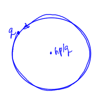
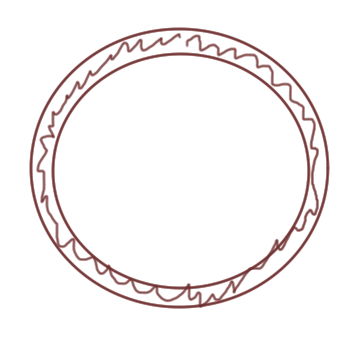
Consider a periodic motion in a fixed ring as sketched in fig. 1.

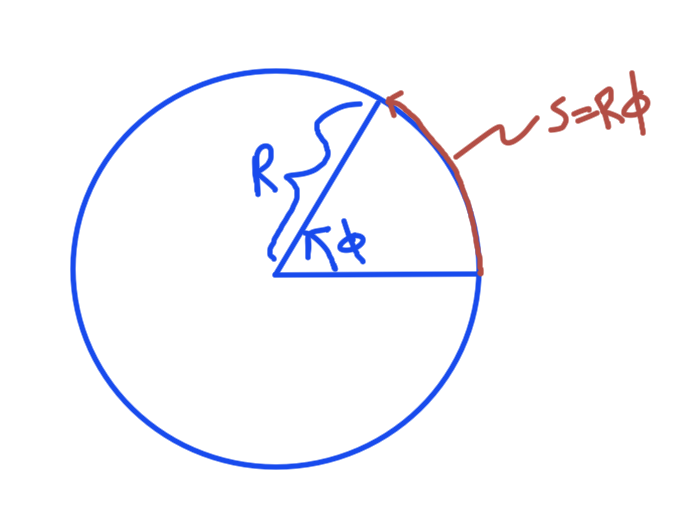
fig. 1. particle confined to a ring

Here the displacement around the perimeter is \( s = R \phi \) and the Hamiltonian

\begin{equation}\label{eqn:qmLecture6:460}
H = – \frac{\Hbar^2}{2 m} \PDSq{s}{} = – \frac{\Hbar^2}{2 m R^2} \PDSq{\phi}{}.
\end{equation}

Now assume that there is a magnetic field squeezed into the point at the origin, by virtue of a flux at the origin

\begin{equation}\label{eqn:qmLecture6:480}
\BB = \Phi_0 \delta(\Br) \zcap.
\end{equation}

We know that

\begin{equation}\label{eqn:qmLecture6:500}
\oint \BA \cdot d\Bl = \Phi_0,
\end{equation}

so that

\begin{equation}\label{eqn:qmLecture6:520}
\BA = \frac{\Phi_0}{2 \pi r} \phicap.
\end{equation}

The Hamiltonian for the new configuration is

\begin{equation}\label{eqn:qmLecture6:540}
\begin{aligned}
H
&= – \lr{ -i \Hbar \spacegrad – q \frac{\Phi_0}{2 \pi r } \phicap }^2 \\
&= – \inv{2 m} \lr{ -i \Hbar \inv{R} \PD{\phi}{} – q \frac{\Phi_0}{2 \pi R } }^2.
\end{aligned}
\end{equation}

Here the replacement \( r \rightarrow R \) makes use of the fact that this problem as been posed with the particle forced to move around the ring at the fixed radius \( R \).

For this transformed Hamiltonian, what are the wave functions?

\begin{equation}\label{eqn:qmLecture6:560}
\psi(\phi)’
\stackrel{?}{=}
e^{i n \phi}.
\end{equation}

\begin{equation}\label{eqn:qmLecture6:580}
\begin{aligned}
H \psi
&= \inv{2 m}
\lr{ -i \Hbar \inv{R} (i n) – q \frac{\Phi_0}{2 \pi R } }^2 e^{i n \phi} \\
&=
\underbrace{\inv{2 m}
\lr{ \frac{\Hbar n}{R} – q \frac{\Phi_0}{2 \pi R } }^2}_{E_n} e^{i n \phi}.
\end{aligned}
\end{equation}

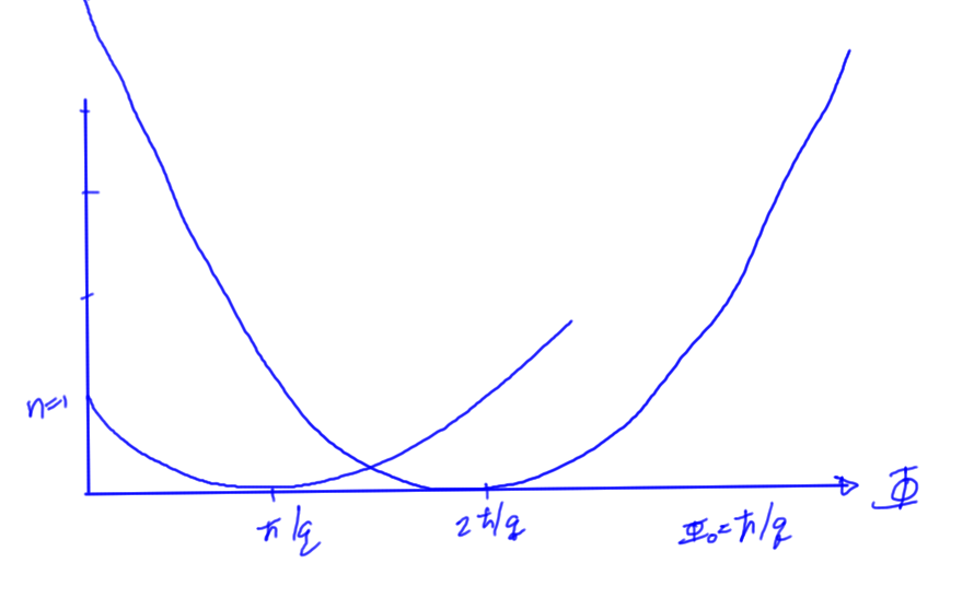
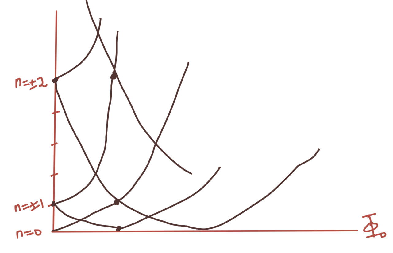
This is very unclassical, since the energy changes in a way that depends on the flux, because particles are seeing magnetic fields that are not present at the point of the particle.

This is sketched in fig. 2.

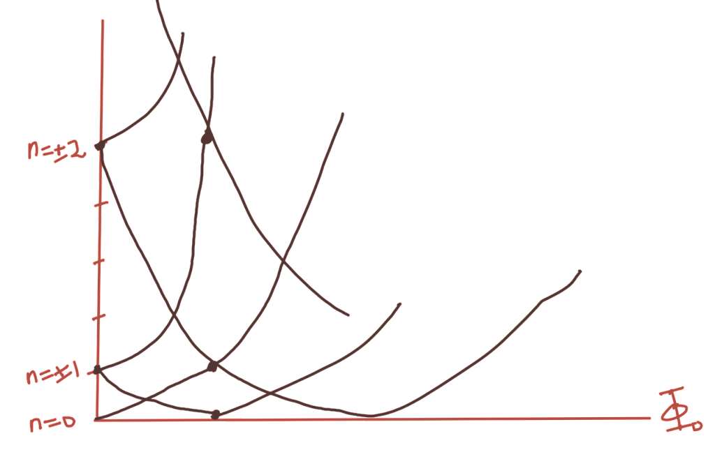
fig. 2. Energy variation with flux.

we see that there are multiple points that the energies hit the minimum levels

Question:

Show that after a transformation of position and momentum of the following form

\begin{equation}\label{eqn:qmLecture6:600}
\begin{aligned}
\hat{\Br}’ &= \hat{\Br} \\
\hat{\Bp}’ &= \hat{\Bp} – q \spacegrad \chi(\Br)
\end{aligned}
\end{equation}

all the commutators have the expected values.

Answer

The position commutators don’t need consideration. Of interest is the momentum-position commutators

\begin{equation}\label{eqn:qmLecture6:620}
\begin{aligned}
\antisymmetric{\hat{p}_k’}{\hat{x}_k’}
&=
\antisymmetric{\hat{p}_k – q \partial_k \chi}{\hat{x}_k} \\
&=
\antisymmetric{\hat{p}_k}{\hat{x}_k} – q \antisymmetric{\partial_k \chi}{\hat{x}_k} \\
&=
\antisymmetric{\hat{p}_k}{\hat{x}_k},
\end{aligned}
\end{equation}

and the momentum commutators

\begin{equation}\label{eqn:qmLecture6:640}
\begin{aligned}
\antisymmetric{\hat{p}_k’}{\hat{p}_j’}
&=
\antisymmetric{\hat{p}_k – q \partial_k \chi}{\hat{p}_j – q \partial_j \chi} \\
&=
\antisymmetric{\hat{p}_k}{\hat{p}_j}
– q \lr{ \antisymmetric{\partial_k \chi}{\hat{p}_j} + \antisymmetric{\hat{p}_k}{\partial_j \chi} }.
\end{aligned}
\end{equation}

That last sum of commutators is

\begin{equation}\label{eqn:qmLecture6:660}
\begin{aligned}
\antisymmetric{\partial_k \chi}{\hat{p}_j} + \antisymmetric{\hat{p}_k}{\partial_j \chi}
&=
– i \Hbar \lr{ \PD{k}{(\partial_j \chi)} – \PD{j}{(\partial_k \chi)} } \\
&= 0.
\end{aligned}
\end{equation}

We’ve shown that

\begin{equation}\label{eqn:qmLecture6:680}
\begin{aligned}
\antisymmetric{\hat{p}_k’}{\hat{x}_k’} &= \antisymmetric{\hat{p}_k}{\hat{x}_k} \\
\antisymmetric{\hat{p}_k’}{\hat{p}_j’} &= \antisymmetric{\hat{p}_k}{\hat{p}_j}.
\end{aligned}
\end{equation}

All the other commutators clearly have the desired transformation properties.

References

[1] Jun John Sakurai and Jim J Napolitano. Modern quantum mechanics. Pearson Higher Ed, 2014.