[Click here for a PDF of this post with nicer formatting]
Disclaimer
Peeter’s lecture notes from class. These may be incoherent and rough.
These are notes for the UofT course ECE1505H, Convex Optimization, taught by Prof. Stark Draper, from [1].
Today
- Local and global optimality
- Compositions of functions
- Examples
Example:
\begin{equation}\label{eqn:convexOptimizationLecture7:20}
\begin{aligned}
F(x) &= x^2 \\
F”(x) &= 2 > 0
\end{aligned}
\end{equation}
strictly convex.
Example:
\begin{equation}\label{eqn:convexOptimizationLecture7:40}
\begin{aligned}
F(x) &= x^3 \\
F”(x) &= 6 x.
\end{aligned}
\end{equation}
Not always non-negative, so not convex. However \( x^3 \) is convex on \( \textrm{dom} F = \mathbb{R}_{+} \).
Example:
\begin{equation}\label{eqn:convexOptimizationLecture7:60}
\begin{aligned}
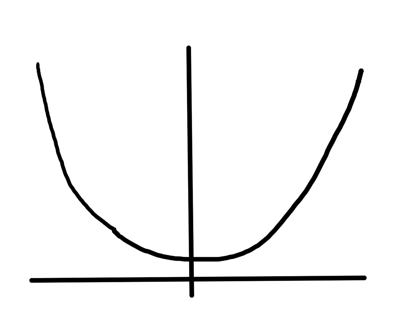
F(x) &= x^\alpha \\
F'(x) &= \alpha x^{\alpha-1} \\
F”(x) &= \alpha(\alpha-1) x^{\alpha-2}.
\end{aligned}
\end{equation}
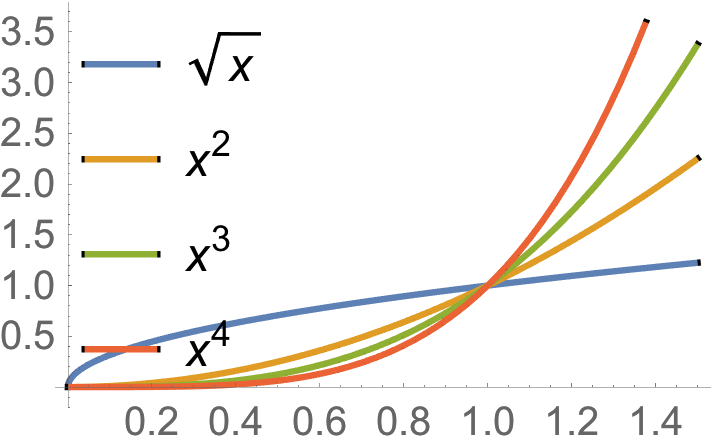
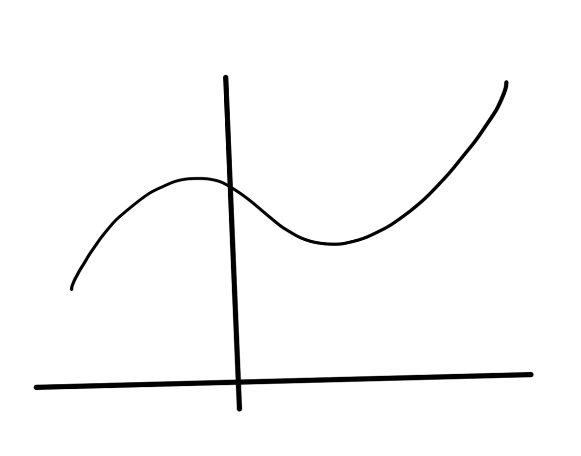
fig. 1. Powers of x.
This is convex on \( \mathbb{R}_{+} \), if \( \alpha \ge 1 \), or \( \alpha \le 0 \).
Example:
\begin{equation}\label{eqn:convexOptimizationLecture7:80}
\begin{aligned}
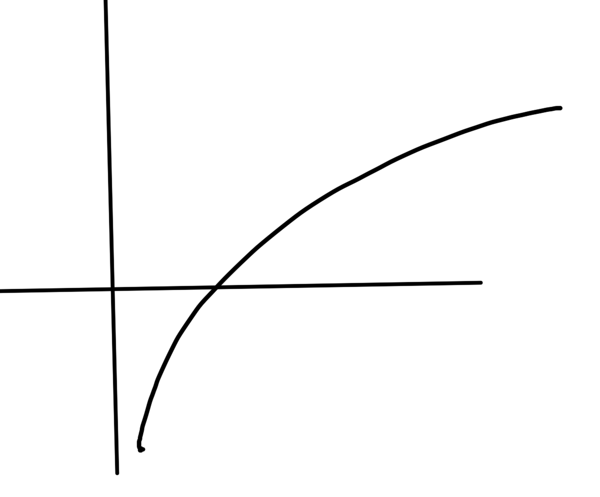
F(x) &= \log x \\
F'(x) &= \inv{x} \\
F”(x) &= -\inv{x^2} \le 0
\end{aligned}
\end{equation}
This is concave.
Example:
\begin{equation}\label{eqn:convexOptimizationLecture7:100}
\begin{aligned}
F(x) &= x\log x \\
F'(x) &= \log x + x \inv{x} = 1 + \log x \\
F”(x) &= \inv{x}
\end{aligned}
\end{equation}
This is strictly convex on
\( \mathbb{R}_{++} \), where
\( F”(x) \ge 0 \).
Example:
\begin{equation}\label{eqn:convexOptimizationLecture7:120}
\begin{aligned}
F(x) &= e^{\alpha x} \\
F'(x) &= \alpha e^{\alpha x} \\
F”(x) &= \alpha^2 e^{\alpha x} \ge 0
\end{aligned}
\end{equation}
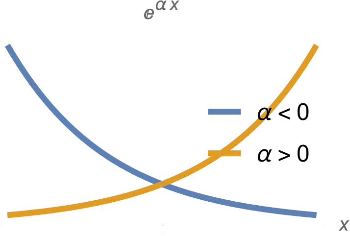
fig. 2. Exponential.
Such functions are plotted in fig. 2, and are convex function for all \( \alpha \).
Example:
For symmetric \( P \in S^n \)
\begin{equation}\label{eqn:convexOptimizationLecture7:140}
\begin{aligned}
F(\Bx) &= \Bx^\T P \Bx + 2 \Bq^\T \Bx + r \\
\spacegrad F &= (P + P^\T) \Bx + 2 \Bq = 2 P \Bx + 2 \Bq \\
\spacegrad^2 F &= 2 P.
\end{aligned}
\end{equation}
This is convex(concave) if \( P \ge 0 \) (\( P \le 0\)).
Example:
A quadratic function
\begin{equation}\label{eqn:convexOptimizationLecture7:780}
F(x, y) = x^2 + y^2 + 3 x y,
\end{equation}
that is neither convex nor concave is plotted in fig 3.
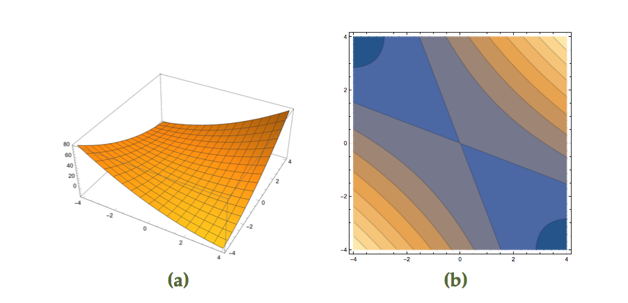
fig 3. Function with saddle point (3d and contours)
This function can be put in matrix form
\begin{equation}\label{eqn:convexOptimizationLecture7:160}
F(x, y) = x^2 + y^2 + 3 x y
=
\begin{bmatrix}
x & y
\end{bmatrix}
\begin{bmatrix}
1 & 1.5 \\
1.5 & 1
\end{bmatrix}
\begin{bmatrix}
x \\
y
\end{bmatrix},
\end{equation}
and has the Hessian
\begin{equation}\label{eqn:convexOptimizationLecture7:180}
\begin{aligned}
\spacegrad^2 F
&=
\begin{bmatrix}
\partial_{xx} F & \partial_{xy} F \\
\partial_{yx} F & \partial_{yy} F \\
\end{bmatrix} \\
&=
\begin{bmatrix}
2 & 3 \\
3 & 2
\end{bmatrix} \\
&= 2 P.
\end{aligned}
\end{equation}
From the plot we know that this is not PSD, but this can be confirmed by checking the eigenvalues
\begin{equation}\label{eqn:convexOptimizationLecture7:200}
\begin{aligned}
0
&=
\det ( P – \lambda I ) \\
&=
(1 – \lambda)^2 – 1.5^2,
\end{aligned}
\end{equation}
which has solutions
\begin{equation}\label{eqn:convexOptimizationLecture7:220}
\lambda = 1 \pm \frac{3}{2} = \frac{3}{2}, -\frac{1}{2}.
\end{equation}
This is not PSD nor negative semi-definite, because it has one positive and one negative eigenvalues. This is neither convex nor concave.
Along \( y = -x \),
\begin{equation}\label{eqn:convexOptimizationLecture7:240}
\begin{aligned}
F(x,y)
&=
F(x,-x) \\
&=
2 x^2 – 3 x^2 \\
&=
– x^2,
\end{aligned}
\end{equation}
so it is concave along this line. Along \( y = x \)
\begin{equation}\label{eqn:convexOptimizationLecture7:260}
\begin{aligned}
F(x,y)
&=
F(x,x) \\
&=
2 x^2 + 3 x^2 \\
&=
5 x^2,
\end{aligned}
\end{equation}
so it is convex along this line.
Example:
\begin{equation}\label{eqn:convexOptimizationLecture7:280}
F(\Bx) = \sqrt{ x_1 x_2 },
\end{equation}
on \( \textrm{dom} F = \setlr{ x_1 \ge 0, x_2 \ge 0 } \)
For the Hessian
\begin{equation}\label{eqn:convexOptimizationLecture7:300}
\begin{aligned}
\PD{x_1}{F} &= \frac{1}{2} x_1^{-1/2} x_2^{1/2} \\
\PD{x_2}{F} &= \frac{1}{2} x_2^{-1/2} x_1^{1/2}
\end{aligned}
\end{equation}
The Hessian components are
\begin{equation}\label{eqn:convexOptimizationLecture7:320}
\begin{aligned}
\PD{x_1}{} \PD{x_1}{F} &= -\frac{1}{4} x_1^{-3/2} x_2^{1/2} \\
\PD{x_1}{} \PD{x_2}{F} &= \frac{1}{4} x_2^{-1/2} x_1^{-1/2} \\
\PD{x_2}{} \PD{x_1}{F} &= \frac{1}{4} x_1^{-1/2} x_2^{-1/2} \\
\PD{x_2}{} \PD{x_2}{F} &= -\frac{1}{4} x_2^{-3/2} x_1^{1/2}
\end{aligned}
\end{equation}
or
\begin{equation}\label{eqn:convexOptimizationLecture7:340}
\spacegrad^2 F
=
-\frac{\sqrt{x_1 x_2}}{4}
\begin{bmatrix}
\inv{x_1^2} & -\inv{x_1 x_2} \\
-\inv{x_1 x_2} & \inv{x_2^2}
\end{bmatrix}.
\end{equation}
Checking this for PSD against \( \Bv = (v_1, v_2) \), we have
\begin{equation}\label{eqn:convexOptimizationLecture7:360}
\begin{aligned}
\begin{bmatrix}
v_1 & v_2
\end{bmatrix}
\begin{bmatrix}
\inv{x_1^2} & -\inv{x_1 x_2} \\
-\inv{x_1 x_2} & \inv{x_2^2}
\end{bmatrix}
\begin{bmatrix}
v_1 \\ v_2
\end{bmatrix}
&=
\begin{bmatrix}
v_1 & v_2
\end{bmatrix}
\begin{bmatrix}
\inv{x_1^2} v_1 -\inv{x_1 x_2} v_2 \\
-\inv{x_1 x_2} v_1 + \inv{x_2^2} v_2
\end{bmatrix} \\
&=
\lr{ \inv{x_1^2} v_1 -\inv{x_1 x_2} v_2 } v_1 +
\lr{ -\inv{x_1 x_2} v_1 + \inv{x_2^2} v_2 } v_2
\\
&=
\inv{x_1^2} v_1^2
+ \inv{x_2^2} v_2^2
-2 \inv{x_1 x_2} v_1 v_2 \\
&=
\lr{
\frac{v_1}{x_1}
-\frac{v_2}{x_2}
}^2 \\
&\ge 0,
\end{aligned}
\end{equation}
so \( \spacegrad^2 F \le 0 \). This is a negative semi-definite function (concave). Observe that this check required checking PSD for all values of \( \Bx \).
This is an example of a more general result
\begin{equation}\label{eqn:convexOptimizationLecture7:380}
F(x) = \lr{ \prod_{i = 1}^n x_i }^{1/n},
\end{equation}
which is concave (prove on homework).
Summary.
If \( F \) is differentiable in \R{n}, then check the curvature of the function along all lines. i.e. At all locations and in all directions.
If the Hessian is PSD at all \( \Bx \in \textrm{dom} F \), that is
\begin{equation}\label{eqn:convexOptimizationLecture7:400}
\spacegrad^2 F \ge 0 \, \forall \Bx \in \textrm{dom} F,
\end{equation}
then the function is convex.
more examples of convex, but not necessarily differentiable functions
Example:
Over \( \textrm{dom} F = \mathbb{R}^n \)
\begin{equation}\label{eqn:convexOptimizationLecture7:420}
F(\Bx) = \max_{i = 1}^n x_i
\end{equation}
i.e.
\begin{equation}\label{eqn:convexOptimizationLecture7:440}
\begin{aligned}
F((1,2) &= 2 \\
F((3,-1) &= 3
\end{aligned}
\end{equation}
Example:
\begin{equation}\label{eqn:convexOptimizationLecture7:460}
F(\Bx) = \max_{i = 1}^n F_i(\Bx),
\end{equation}
where
\begin{equation}\label{eqn:convexOptimizationLecture7:480}
F_i(\Bx)
=
… ?
\end{equation}
max of a set of convex functions is a convex function.
Example:
\begin{equation}\label{eqn:convexOptimizationLecture7:500}
F(x) =
x_{[1]} +
x_{[2]} +
x_{[3]}
\end{equation}
where
\( x_{[k]} \) is the k-th largest number in the list
Write
\begin{equation}\label{eqn:convexOptimizationLecture7:520}
F(x) = \max x_i + x_j + x_k
\end{equation}
\begin{equation}\label{eqn:convexOptimizationLecture7:540}
(i,j,k) \in \binom{n}{3}
\end{equation}
Example:
For \( \Ba \in \mathbb{R}^n \) and \( b_i \in \mathbb{R} \)
\begin{equation}\label{eqn:convexOptimizationLecture7:560}
\begin{aligned}
F(\Bx)
&= \sum_{i = 1}^n \log( b_i – \Ba^\T \Bx )^{-1} \\
&= -\sum_{i = 1}^n \log( b_i – \Ba^\T \Bx )
\end{aligned}
\end{equation}
This \( b_i – \Ba^\T \Bx \) is an affine function of \( \Bx \) so it doesn’t affect convexity.
Since \( \log \) is concave, \( -\log \) is convex. Convex functions of affine function of \( \Bx \) is convex function of \( \Bx \).
Example:
\begin{equation}\label{eqn:convexOptimizationLecture7:580}
F(\Bx) = \sup_{\By \in C} \Norm{ \Bx – \By }
\end{equation}
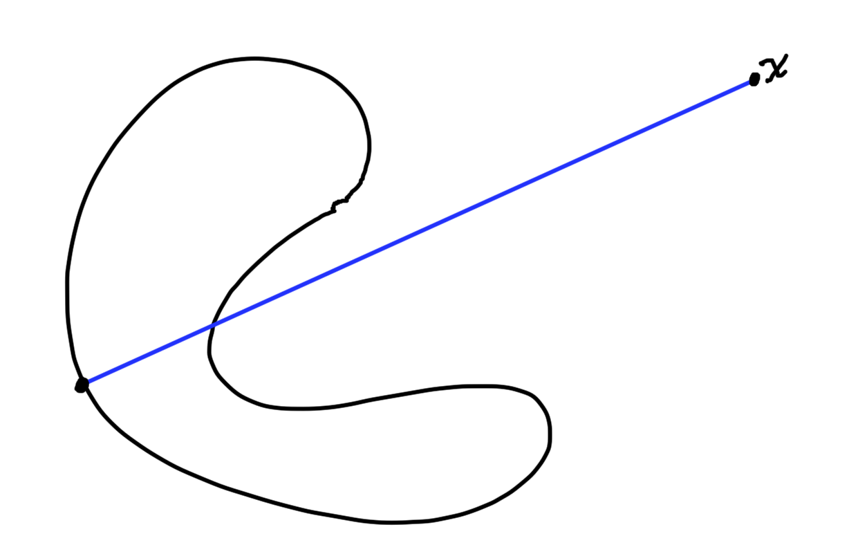
fig. 3. Max length function
Here \( C \subseteq \mathbb{R}^n \) is not necessarily convex. We are using \( \sup \) here because the set \( C \) may be open. This function is the length of the line from \( \Bx \) to the point in \( C \) that is furthest from \( \Bx \).
- \( \Bx – \By \) is linear in \( \Bx \)
- \( g_\By(\Bx) = \Norm{\Bx – \By} \) is convex in \( \Bx \) since norms are convex functions.
- \( F(\Bx) = \sup_{\By \in C} \Norm{ \Bx – \By } \). Each \( \By \) index is a convex function. Taking max of those.
Example:
\begin{equation}\label{eqn:convexOptimizationLecture7:600}
F(\Bx) = \inf_{\By \in C} \Norm{ \Bx – \By }.
\end{equation}
Min and max of two convex functions are plotted in fig. 4.
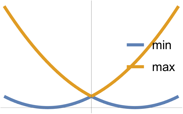
fig. 4. Min and max
The max is observed to be convex, whereas the min is not necessarily so.
\begin{equation}\label{eqn:convexOptimizationLecture7:800}
F(\Bz) = F(\theta \Bx + (1-\theta) \By) \ge \theta F(\Bx) + (1-\theta)F(\By).
\end{equation}
This is not necessarily convex for all sets \( C \subseteq \mathbb{R}^n \), because the \( \inf \) of a bunch of convex function is not necessarily convex. However, if \( C \) is convex, then \( F(\Bx) \) is convex.
Consequences of convexity for differentiable functions
- Think about unconstrained functions \( \textrm{dom} F = \mathbb{R}^n \).
- By first order condition \( F \) is convex iff the domain is convex and
\begin{equation}\label{eqn:convexOptimizationLecture7:620}
F(\Bx) \ge \lr{ \spacegrad F(\Bx)}^\T (\By – \Bx) \, \forall \Bx, \By \in \textrm{dom} F.
\end{equation}
If \( F \) is convex and one can find an \( \Bx^\conj \in \textrm{dom} F \) such that
\begin{equation}\label{eqn:convexOptimizationLecture7:640}
\spacegrad F(\Bx^\conj) = 0,
\end{equation}
then
\begin{equation}\label{eqn:convexOptimizationLecture7:660}
F(\By) \ge F(\Bx^\conj) \, \forall \By \in \textrm{dom} F.
\end{equation}
If you can find the point where the gradient is zero (which can’t always be found), then \( \Bx^\conj\) is a global minimum of \( F \).
Conversely, if \( \Bx^\conj \) is a global minimizer of \( F \), then \( \spacegrad F(\Bx^\conj) = 0 \) must hold. If that were not the case, then you would be able to find a direction to move downhill, contracting the optimality of \( \Bx^\conj\).
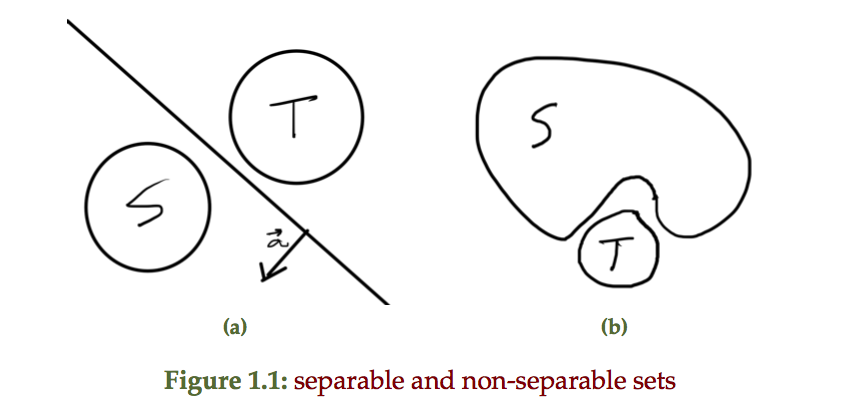
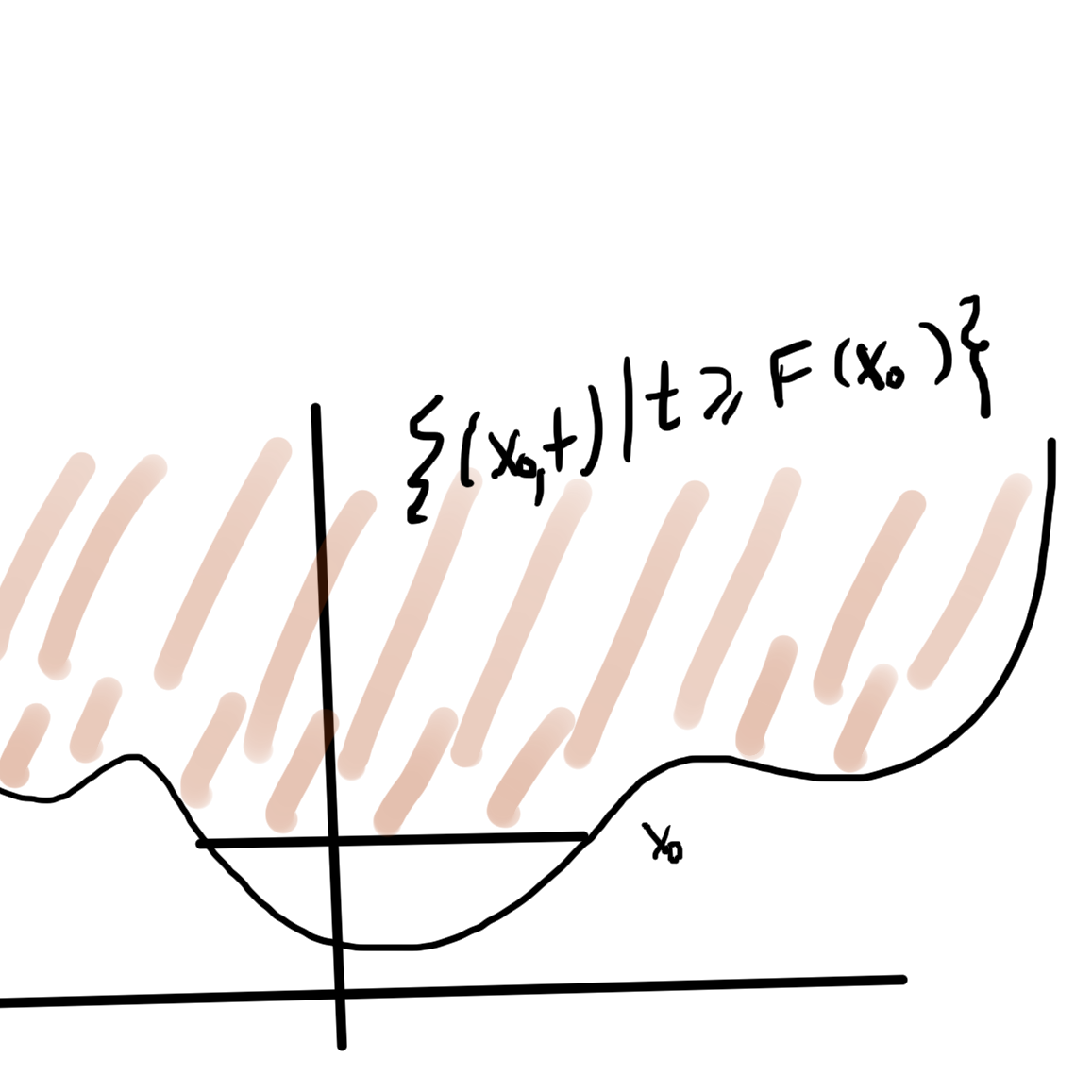
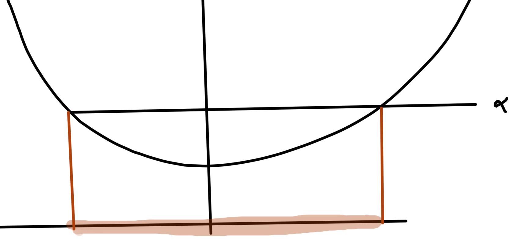
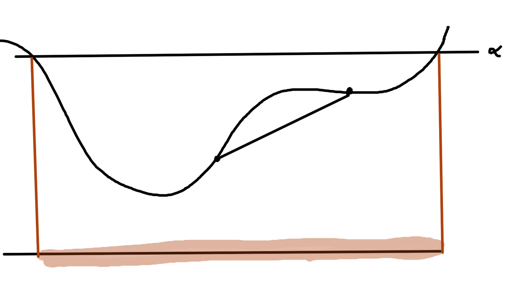
Local vs Global optimum
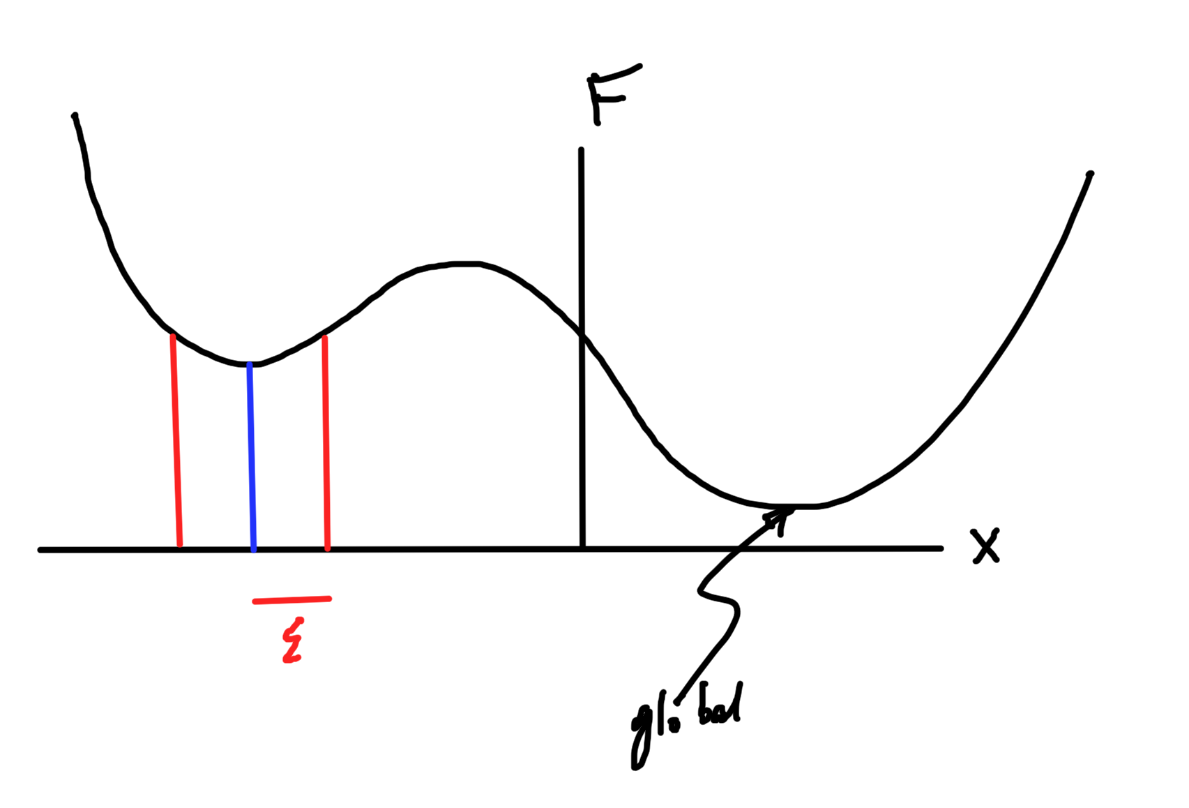
fig. 6. Global and local minimums
Definition: Local optimum
\( \Bx^\conj \) is a local optimum of \( F \) if \( \exists \epsilon > 0 \) such that \( \forall \Bx \), \( \Norm{\Bx – \Bx^\conj} < \epsilon \), we have
\begin{equation*}
F(\Bx^\conj) \le F(\Bx)
\end{equation*}
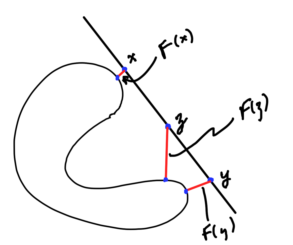
fig. 5. min length function
Theorem:
Suppose \( F \) is twice continuously differentiable (not necessarily convex)
- If \( \Bx^\conj\) is a local optimum then\begin{equation*}
\begin{aligned}
\spacegrad F(\Bx^\conj) &= 0 \\
\spacegrad^2 F(\Bx^\conj) \ge 0
\end{aligned}
\end{equation*} - If
\begin{equation*}
\begin{aligned}
\spacegrad F(\Bx^\conj) &= 0 \\
\spacegrad^2 F(\Bx^\conj) \ge 0
\end{aligned},
\end{equation*}then \( \Bx^\conj\) is a local optimum.
Proof:
- Let \( \Bx^\conj \) be a local optimum. Pick any \( \Bv \in \mathbb{R}^n \).\begin{equation}\label{eqn:convexOptimizationLecture7:720}
\lim_{t \rightarrow 0} \frac{ F(\Bx^\conj + t \Bv) – F(\Bx^\conj)}{t}
= \lr{ \spacegrad F(\Bx^\conj) }^\T \Bv
\ge 0.
\end{equation}
Here the fraction is \( \ge 0 \) since \( \Bx^\conj \) is a local optimum.
Since the choice of \( \Bv \) is arbitrary, the only case that you can ensure that \( \ge 0, \forall \Bv \) is
\begin{equation}\label{eqn:convexOptimizationLecture7:740}
\spacegrad F = 0,
\end{equation}
( or else could pick \( \Bv = -\spacegrad F(\Bx^\conj) \).
This means that \( \spacegrad F(\Bx^\conj) = 0 \) if \( \Bx^\conj \) is a local optimum.
Consider the 2nd order derivative
\begin{equation}\label{eqn:convexOptimizationLecture7:760}
\begin{aligned}
\lim_{t \rightarrow 0} \frac{ F(\Bx^\conj + t \Bv) – F(\Bx^\conj)}{t^2}
&=
\lim_{t \rightarrow 0} \inv{t^2}
\lr{
F(\Bx^\conj) + t \lr{ \spacegrad F(\Bx^\conj) }^\T \Bv + \inv{2} t^2 \Bv^\T \spacegrad^2 F(\Bx^\conj) \Bv + O(t^3)
– F(\Bx^\conj)
} \\
&=
\inv{2} \Bv^\T \spacegrad^2 F(\Bx^\conj) \Bv \\
&\ge 0.
\end{aligned}
\end{equation}
Here the \( \ge \) condition also comes from the fraction, based on the optimiality of \( \Bx^\conj \). This is true for all choice of \( \Bv \), thus \( \spacegrad^2 F(\Bx^\conj) \).
References
[1] Stephen Boyd and Lieven Vandenberghe. Convex optimization. Cambridge university press, 2004.