creation operator

PHY2403: QFT I: Momentum of scalar field: time dependent terms?

November 8, 2018 phy2403 , , ,

[Click here for a PDF of this post with nicer formatting]

Way back in lecture 8, it was claimed that
\begin{equation}\label{eqn:momentum:20}
P^k = \int d^3 x \hat{\pi} \partial^k \hat{\phi} = \int \frac{d^3 p}{(2\pi)^3} p^k a_\Bp^\dagger a_\Bp.
\end{equation}
If I compute this, I get a normal ordered variation of this operator, but also get some time dependent terms. Here’s the computation (dropping hats)
\begin{equation}\label{eqn:momentum:40}
\begin{aligned}
P^k
&= \int d^3 x \hat{\pi} \partial^k \phi \\
&= \int d^3 x \partial_0 \phi \partial^k \phi \\
&= \int d^3 x \frac{d^3 p d^3 q}{(2 \pi)^6} \inv{\sqrt{2 \omega_p 2 \omega_q} }
\partial_0
\lr{
a_\Bp e^{-i p \cdot x}
+
a_\Bp^\dagger e^{i p \cdot x}
}
\partial^k
\lr{
a_\Bq e^{-i q \cdot x}
+
a_\Bq^\dagger e^{i q \cdot x}
}.
\end{aligned}
\end{equation}
The exponential derivatives are
\begin{equation}\label{eqn:momentum:60}
\begin{aligned}
\partial_0 e^{\pm i p \cdot x}
&=
\partial_0 e^{\pm i p_\mu x^\mu} \\
&=
\pm i p_0
\partial_0 e^{\pm i p \cdot x},
\end{aligned}
\end{equation}
and
\begin{equation}\label{eqn:momentum:80}
\begin{aligned}
\partial^k e^{\pm i p \cdot x}
&=
\partial^k e^{\pm i p^\mu x_\mu} \\
&=
\pm i p^k e^{\pm i p \cdot x},
\end{aligned}
\end{equation}
so
\begin{equation}\label{eqn:momentum:100}
\begin{aligned}
P^k
&=
-\int d^3 x \frac{d^3 p d^3 q}{(2 \pi)^6} \inv{\sqrt{2 \omega_p 2 \omega_q} }
p_0 q^k
\lr{
-a_\Bp e^{-i p \cdot x}
+
a_\Bp^\dagger e^{i p \cdot x}
}
\lr{
-a_\Bq e^{-i q \cdot x}
+
a_\Bq^\dagger e^{i q \cdot x}
} \\
&=
-\inv{2} \int d^3 x \frac{d^3 p d^3 q}{(2 \pi)^6} \sqrt{\frac{\omega_p}{\omega_q}} q^k
\lr{
a_\Bp a_\Bq e^{-i (p + q) \cdot x}
+ a_\Bp^\dagger a_\Bq^\dagger e^{i (p + q) \cdot x}
– a_\Bp a_\Bq^\dagger e^{i (q – p) \cdot x}
– a_\Bp^\dagger a_\Bq e^{i (p – q) \cdot x}
} \\
&=
\inv{2} \int \frac{d^3 p d^3 q}{(2 \pi)^3} \sqrt{\frac{\omega_p}{\omega_q}} q^k
\lr{
– a_\Bp a_\Bq e^{- i(\omega_\Bp + \omega_\Bq) t} \delta^3(\Bp + \Bq)
– a_\Bp^\dagger a_\Bq^\dagger e^{i(\omega_\Bp + \omega_\Bq) t} \delta^3(-\Bp – \Bq)
+ a_\Bp a_\Bq^\dagger e^{i(\omega_\Bq – \omega_\Bp) t} \delta^3(\Bp – \Bq)
+ a_\Bp^\dagger a_\Bq e^{i(\omega_\Bp – \omega_\Bq) t} \delta^3(\Bq – \Bp)
} \\
&=
\inv{2} \int \frac{d^3 p }{(2 \pi)^3} p^k
\lr{
a_\Bp^\dagger a_\Bp
+ a_\Bp a_\Bp^\dagger
– a_\Bp a_{-\Bp} e^{- 2 i \omega_\Bp t}
– a_\Bp^\dagger a_{-\Bp}^\dagger e^{2 i \omega_\Bp t}
}.
\end{aligned}
\end{equation}

What is the rationale for ignoring those time dependent terms? Does normal ordering also implicitly drop any non-paired creation/annihilation operators? If so, why?

PHY2403H Quantum Field Theory. Lecture 10: Lorentz boosts, generator of spacetime translation, Lorentz invariant field representation. Taught by Prof. Erich Poppitz

October 16, 2018 phy2403 , , , , ,

[Click here for a PDF of this post with nicer formatting]

DISCLAIMER: Very rough notes from class, with some additional side notes.

These are notes for the UofT course PHY2403H, Quantum Field Theory I, taught by Prof. Erich Poppitz fall 2018.

Lorentz transform symmetries.

From last time, recall that an infinitesimal Lorentz transform has the form
\begin{equation}\label{eqn:qftLecture10:20}
x^\mu \rightarrow x^\mu + \omega^{\mu\nu} x_\nu,
\end{equation}
where
\begin{equation}\label{eqn:qftLecture10:40}
\omega^{\mu\nu} = -\omega^{\nu\mu}
\end{equation}

We showed last time that \( \omega^{ij} \) induces a rotation, and will show today that \( \omega^{0i} \) is a boost.

We introduced a three index current, factoring out explicit dependence on the incremental Lorentz transform tensor \( \omega^{\mu\nu} \) as follows
\begin{equation}\label{eqn:qftLecture10:80}
J^{\nu \mu\rho} = \inv{2} \lr{ x^\rho T^{\nu\mu} – x^\mu T^{\nu\rho} },
\end{equation}
and can easily show that this current has the desired zero four-divergence property
\begin{equation}\label{eqn:qftLecture10:100}
\begin{aligned}
\partial_\nu J^{\nu \mu\rho}
&= \inv{2} \lr{
(\partial_\nu x^\rho) T^{\nu\mu}
+
x^\rho {\partial_\nu T^{\nu\mu} }
– (\partial_\nu x^\mu) T^{\nu\rho}
– x^\mu {\partial_\nu T^{\nu\rho} }
} \\
&= \inv{2} \lr{
(\partial_\nu x^\rho) T^{\nu\mu}
– (\partial_\nu x^\mu) T^{\nu\rho}
} \\
&= \inv{2} \lr{
T^{\rho\mu}
+
– T^{\mu\rho}
} \\
&= 0,
\end{aligned}
\end{equation}
since the energy-momentum tensor is symmetric.

Defining charge in the usual fashion \( Q = \int d^3 x j^0 \), so we can define a charge for each pair of indexes \( \mu\nu \), and in particular
\begin{equation}\label{eqn:qftLecture10:120}
Q^{0k} = \int d^3 x J^{0 0 k} = \inv{2} \int d^3 x \lr{ x^k T^{00} – x^0 T^{0k} }
\end{equation}
\begin{equation}\label{eqn:qftLecture10:540}
\begin{aligned}
\dot{Q}^{0k}
&= \int d^3 x \dot{J}^{0 0k} \\
&= \inv{2} \int d^3 x \lr{ x^k \dot{T}^{00} – x^0 \dot{T}^{0k} }
\end{aligned}
\end{equation}

However, since \( 0 = \partial_\mu T^{\mu \nu} = \dot{T}^{0 \nu} + \partial_j T^{j \nu} \), or \( \dot{T}^{0 \nu} = -\partial_j T^{j \nu} \),
\begin{equation}\label{eqn:qftLecture10:560}
\begin{aligned}
\dot{Q}^{0k}
&= \inv{2} \int d^3 x \lr{ x^k (-\partial_j T^{j0}) – T^{0k} – x^0 (-\partial_j T^{jk}) } \\
&= \inv{2} \int d^3 x \lr{
\partial_j (-x^k T^{j0}) + (\partial_j x^k) T^{j0}
– T^{0k} + x^0 \partial_j T^{jk}
} \\
&= \inv{2} \int d^3 x \lr{
\partial_j (-x^k T^{j0}) + {T^{k0}}
– {T^{0k}} + x^0 \partial_j T^{jk}
} \\
&= \inv{2} \int d^3 x \lr{
\partial_j (-x^k T^{j0})
+ x^0 \partial_j T^{jk}
} \\
&= \inv{2} \int d^3 x
\partial_j \lr{
-x^k T^{j0}
+ x^0 T^{jk}
},
\end{aligned}
\end{equation}
which leaves just surface terms, so \( \dot{Q}^{0k} = 0 \).

Quantizing:

From our previous identification
\begin{equation}\label{eqn:qftLecture9:560}

{T^\nu}_\mu =
-\partial^\nu \phi \partial_\mu \phi + {\delta^{\nu}}_\mu \LL,
\end{equation}
we have
\begin{equation}\label{eqn:qftLecture10:580}
T^{\nu\mu} = \partial^\nu \phi \partial^\mu \phi – g^{\nu\mu} \LL,
\end{equation}
or
\begin{equation}\label{eqn:qftLecture10:600}
\begin{aligned}
T^{00}
&= \partial^0 \phi \partial^0 \phi – \inv{2} \lr{ \partial_0 \phi \partial^0 \phi + \partial_k \phi \partial^k \phi } \\
&= \inv{2} \partial^0 \phi \partial^0 \phi – \inv{2} (\spacegrad \phi)^2,
\end{aligned}
\end{equation}
and
\begin{equation}\label{eqn:qftLecture10:620}
T^{0k} = \partial^0 \phi \partial^k \phi,
\end{equation}
so we may quantize these energy momentum tensor components as
\begin{equation}\label{eqn:qftLecture10:640}
\begin{aligned}
\hatT^{00} &= \inv{2} \hat{\pi}^2 + \inv{2} (\spacegrad \phihat)^2 \\
\hatT^{0k} &= \inv{2} \hat{\pi} \partial^k \phihat.
\end{aligned}
\end{equation}

We can now start computing the commutators associated with the charge operator. The first of those commutators is
\begin{equation}\label{eqn:qftLecture10:140}
\antisymmetric{\hatT^{00}(\Bx)}{\phihat(\By)}
=
\inv{2}
\antisymmetric{\hat{\pi}^2(\Bx)}{\phihat(\By)},
\end{equation}
which can be evaluated using the field commutator analogue of \( \antisymmetric{F(p)}{q} = i F’ \) which is
\begin{equation}\label{eqn:qftLecture10:660}
\antisymmetric{F(\hat{\pi}(\Bx))}{\phihat(\By)} = -i \frac{dF}{d \hat{\pi}} \delta(\Bx – \By),
\end{equation}
to give
\begin{equation}\label{eqn:qftLecture10:680}
\antisymmetric{\hatT^{00}(\Bx)}{\phihat(\By)}
= -i \delta^3(\Bx – \By) \hat{\pi}(\Bx)
\end{equation}

The other required commutator is
\begin{equation}\label{eqn:qftLecture10:160}
\begin{aligned}
\antisymmetric{\hatT^{0i}(\Bx)}{\phihat(\By)}
&=
\antisymmetric{\hat{\pi}(\Bx)\partial^i \phihat(\Bx)}{\phihat(\By)} \\
&=
\partial^i \phihat(\Bx)
\antisymmetric{\hat{\pi}(\Bx)
}{\phihat(\By)} \\
&= -i \delta^3(\Bx – \By) \partial^i \phihat(\Bx),
\end{aligned}
\end{equation}

The charge commutator with the field can now be computed
\begin{equation}\label{eqn:qftLecture10:180}
\begin{aligned}
i \epsilon \antisymmetric{\hatQ^{0k}}{\phihat(\By)}
&=
i
\frac{\epsilon}{2} \int d^3 x
\lr{
x^k
\antisymmetric{\hatT^{00}}{\phihat(\By)}

x^0
\antisymmetric{\hatT^{0k}}{\phihat(\By)}
} \\
&=
\frac{\epsilon}{2} \lr{ y^k \hat{\pi}(\By) – y^0 \partial^k \phihat(\By) } \\
&=
\frac{\epsilon}{2} \lr{ y^k \dot{\phihat}(\By) – y^0 \partial^k \phihat(\By) },
\end{aligned}
\end{equation}
so to first order in \( \epsilon \)
\begin{equation}\label{eqn:qftLecture10:200}
e^{i \epsilon \hatQ^{0k} } \phihat(\By)
e^{-i \epsilon \hatQ^{0k} }
=
\phihat(\By)
+ \frac{\epsilon}{2} y^k \dot{\phihat}(\By)
+ \frac{\epsilon}{2} y^0 \partial_k \phihat(\By)
\end{equation}

For example, with \( k = 1 \)
\begin{equation}\label{eqn:qftLecture10:700}
\begin{aligned}
e^{i \epsilon \hatQ^{0k} } \phihat(\By)
e^{-i \epsilon \hatQ^{0k} }
&=
\phihat(\By)
+ \frac{\epsilon}{2} \lr{
y^1 \dot{\phihat}(\By)
+
y^0 \PD{y^1}{\phihat}(\By)
} \\
&=
\phihat(y^0 + \frac{\epsilon}{2} y^1,
y^1 + \frac{\epsilon}{2} y^2, y^3).
\end{aligned}
\end{equation}

This is a boost. If we compare explicitly to an infinitesimal Lorentz transformation of the coordinates
\begin{equation}\label{eqn:qftLecture10:220}
\begin{aligned}
x^0 \rightarrow x^0 + \omega^{01} x_1 &= x^0 – \omega^{01} x^1 \\
x^1 \rightarrow x^1 + \omega^{10} x_0 &= x^1 – \omega^{01} x_0 = x^1 – \omega^{01} x^0
\end{aligned}
\end{equation}
we can make the identification
\begin{equation}\label{eqn:qftLecture10:240}
\frac{\epsilon}{2} = – \omega^{01}.
\end{equation}

We now have the explicit form of the generator of a spacetime translation

\begin{equation}\label{eqn:qftLecture10:260}
\boxed{
\hatU(\Lambda) = \exp\lr{-i \omega^{0k} \int d^3 x \lr{ \hatT^{00} x^k – \hatT^{0k} x^0 }}
}
\end{equation}

An explicit boost along the x-axis has the form
\begin{equation}\label{eqn:qftLecture10:300}
\hatU(\Lambda) \phihat(t, \Bx)
\hatU^\dagger(\Lambda)
=
\phihat\lr{ \frac{t – vx}{\sqrt{1 – v^2}}, \frac{x – vt}{\sqrt{1 – v^2}}, y, z },
\end{equation}
and more generally
\begin{equation}\label{eqn:qftLecture10:320}
\hatU(\Lambda) \phihat(x) \hatU^\dagger(\Lambda) =
\phihat(\Lambda x)
\end{equation}
where \( x \) is a four vector, \( (\Lambda x)^\mu = {{\Lambda}^\mu}_\nu x^\nu \), and \(
{{\Lambda}^\mu}_\nu
\approx
{{\delta}^\mu}_\nu
+
{{\omega}^\mu}_\nu \).

Transformation of momentum states

In the momentum space representation

\begin{equation}\label{eqn:qftLecture10:340}
\begin{aligned}
\phihat(x)
&=
\int \frac{d^3 p}{(2 \pi)^3 \sqrt{2 \omega_\Bp}} \lr{
e^{i (\omega_\Bp t – \Bp \cdot \Bx)} \hat{a}_\Bp
+
e^{-i (\omega_\Bp t – \Bp \cdot \Bx)} \hat{a}^\dagger_\Bp
} \\
&=
\int \frac{d^3 p}{(2 \pi)^3 \sqrt{2 \omega_\Bp}} \evalbar{
\lr{
e^{i p^\mu x^\mu } \hat{a}_\Bp
+
e^{-i p^\mu x^\mu } \hat{a}^\dagger_\Bp
}
}{p_0 = \omega_\Bp}
\end{aligned}
\end{equation}
\begin{equation}\label{eqn:qftLecture10:720}
\begin{aligned}
\hatU(\Lambda) \phihat(x) \hatU^\dagger(\Lambda)
&=
\phihat(\Lambda x) \\
&=
\int \frac{d^3 p}{(2 \pi)^3 \sqrt{2 \omega_\Bp}} \evalbar{
\lr{
e^{i p^\mu {{\Lambda}^\mu}_\nu x^\nu }
\hat{a}_\Bp
+
e^{-i p^\mu {{\Lambda}^\mu}_\nu x^\nu } \hat{a}^\dagger_\Bp
}
}{p_0 = \omega_\Bp}
\end{aligned}
\end{equation}
This can be put into an explicitly Lorentz invariant form
\begin{equation}\label{eqn:qftLecture10:n}
\begin{aligned}
\phihat(\Lambda x)
&=
\int \frac{dp^0 d^3 p}{(2\pi)^3} \delta(p_0^2 – \Bp^2 – m^2) \Theta(p^0) \sqrt{2 \omega_\Bp}
e^{i p^\mu {{\Lambda}^\mu}_\nu x^\nu }
\hat{a}_\Bp + \text{h.c.} \\
&=
\int \frac{dp^0 d^3 p}{(2\pi)^3}
\lr{
\frac{\delta(p_0 – \omega_\Bp)}{2 \omega_\Bp}
+
\frac{\delta(p_0 + \omega_\Bp)}{2 \omega_\Bp}
}
\Theta(p^0) \sqrt{2 \omega_\Bp} \hat{a}_\Bp + \text{h.c.},
\end{aligned}
\end{equation}
which recovers \ref{eqn:qftLecture10:720} by making use of the delta function identity \( \delta(f(x)) = \sum_{f(x_\conj) = 0} \frac{\delta(x – x_\conj)}{f'(x_\conj)} \), since the \( \Theta(p^0) \) kills the second delta function.

We now have a more explicit Lorentz invariant structure
\begin{equation}\label{eqn:qftLecture10:380}
\phihat(\Lambda x)
=
\int \frac{dp^0 d^3 p}{(2\pi)^3} \delta(p_0^2 – \Bp^2 – m^2) \Theta(p^0) \sqrt{2 \omega_\Bp}
e^{i p^\mu {{\Lambda}^\mu}_\nu x^\nu }
\hat{a}_\Bp + \text{h.c.}
\end{equation}

Recall that a boost moves a spacetime point along a parabola, such as that of fig. 1, whereas a rotation moves along a constant “circular” trajectory of a hyper-paraboloid. In general, a Lorentz transformation may move a spacetime point along any path on a hyper-paraboloid such as the one depicted (in two spatial dimensions) in fig. 2. This paraboloid depict the surfaces of constant energy-momentum \( p^0 = \sqrt{ \Bp^2 + m^2 } \). Because a Lorentz transformation only shift points along that energy-momentum surface, but cannot change the sign of the energy coordinate \( p^0 \), this means that \( \Theta(p^0) \) is also a Lorentz invariant.

fig. 1. One dimensional spacetime surface for constant (p^0)^2 – p^2 = m^2.


fig. 2. Surface of constant squared four-momentum.


Let’s change variables
\begin{equation}\label{eqn:qftLecture10:400}
p^\lambda = {{\Lambda}^\lambda}_\rho {p’}^{\rho}
\end{equation}
so that
\begin{equation}\label{eqn:qftLecture10:420}
\begin{aligned}
p_\mu
{{\Lambda}^\mu}_\nu x^\nu
&=
{{\Lambda}^\lambda}_\rho {p’}^\rho g_{\lambda\nu} {{\Lambda}^\nu}_\sigma x^{\sigma} \\
&=
{p’}^\rho
\lr{ {{\Lambda}^\lambda}_\rho
g_{\lambda\nu} {{\Lambda}^\nu}_\sigma } x^{\sigma} \\
&=
{p’}^\rho g_{\rho\sigma} x^\sigma
\end{aligned}
\end{equation}
which gives
\begin{equation}\label{eqn:qftLecture10:440}
\begin{aligned}
\phihat(\Lambda x)
&=
\int \frac{d{p’}^0 d^3 p’}{(2\pi)^3} \delta({p’}_0^2 – {\Bp’}^2 – m^2) \Theta(p^0) \sqrt{2 \omega_{\Lambda \Bp’}} e^{i p’ \cdot x} \hat{a}_{\Lambda \Bp’} + \text{h.c.} \\
&=
\int \frac{dp^0 d^3 p}{(2\pi)^3} \delta({p}_0^2 – {\Bp}^2 – m^2) \Theta(p^0) \sqrt{2 \omega_{\Lambda \Bp}} e^{i p \cdot x} \hat{a}_{\Lambda \Bp} + \text{h.c.}
\end{aligned}
\end{equation}
Since
\begin{equation}\label{eqn:qftLecture10:460}
\phihat(x)
=
\int \frac{dp^0 d^3 p}{(2\pi)^3} \delta({p}_0^2 – {\Bp}^2 – m^2) \Theta(p^0) \sqrt{2 \omega_{\Bp}} e^{i p \cdot x} \hat{a}_{\Bp} + \text{h.c.}
\end{equation}
we can now conclude that the creation and annihilation operators transform as

\begin{equation}\label{eqn:qftLecture10:480}
\boxed{
\sqrt{2 \omega_{\Lambda \Bp}} \hat{a}_{\Lambda \Bp}
=
\hatU(\Lambda)
\sqrt{2 \omega_{ \Bp}} \hat{a}_{ \Bp}
\hatU^\dagger(\Lambda)
}
\end{equation}

In particular
\begin{equation}\label{eqn:qftLecture10:500}
\sqrt{2 \omega_{ \Bp}} \hat{a}^\dagger_{ \Bp} \ket{0} = \ket{\Bp}
\end{equation}
and noting that \( \hatU(\Lambda) \ket{0} = \ket{0} \) (i.e. the ground state is Lorentz invariant), we have
\begin{equation}\label{eqn:qftLecture10:520}
\begin{aligned}
\sqrt{2 \omega_{\Lambda \Bp}} \hat{a}^\dagger_{\Lambda \Bp} \ket{0}
&=
\hatU(\Lambda) \sqrt{ 2\omega_\Bp} \hat{a}^\dagger_\Bp \hatU^\dagger(\Lambda) \hatU(\Lambda) \ket{0} \\
&=
\hatU(\Lambda) \sqrt{ 2\omega_\Bp} \hat{a}^\dagger_\Bp \ket{0} \\
&=
\hatU(\Lambda) \ket{\Bp}.
\end{aligned}
\end{equation}

PHY2403H Quantum Field Theory. Lecture 6: Canonical quantization, Simple Harmonic Oscillators, Symmetries. Taught by Prof. Erich Poppitz

September 26, 2018 phy2403 , , ,

[Click here for a PDF of this post with nicer formatting]

DISCLAIMER: Very rough notes from class, with some additional side notes (QM SHO review, …).

These are notes for the UofT course PHY2403H, Quantum Field Theory I, taught by Prof. Erich Poppitz fall 2018.

Quantization of Field Theory

We are engaging in the “canonical” or Hamiltonian method of quantization. It is also possible to quantize using path integrals, but it is hard to prove that operators are unitary doing so. In fact, the mechanism used to show unitarity from path integrals is often to find the Lagrangian and show that there is a Hilbert space (i.e. using canonical quantization). Canonical quantization essentially demands that the fields obey a commutator relation of the following form
\begin{equation}\label{eqn:qftLecture6:20}
\antisymmetric{\pi(\Bx, t)}{\phi(\By, t)} = -i \delta^3(\Bx – \By).
\end{equation}
We assumed that the quantized fields obey the Hamiltonian relations
\begin{equation}\label{eqn:qftLecture6:160}
\begin{aligned}
\ddt{\phi} &= i \antisymmetric{H}{\phi} \\
\ddt{\pi} &= i \antisymmetric{H}{\pi}.
\end{aligned}
\end{equation}

We were working with the Hamiltonian density
\begin{equation}\label{eqn:qftLecture6:40}
\mathcal{H} =
\inv{2} (\pi(\Bx, t))^2
+
\inv{2} (\spacegrad \phi(\Bx, t))^2
+
\frac{m^2}{2} \phi^2
+
\frac{\lambda}{4} \phi^4,
\end{equation}
which included a mass term \( m \) and a potential term (\(\lambda\)). We will expand all quantities in Taylor series in \( \lambda \) assuming they have a structure such as
\begin{equation}\label{eqn:qftLecture6:180}
\begin{aligned}
f(\lambda) =
c_0 \lambda^0
+ c_1 \lambda^1
+ c_2 \lambda^2
+ c_3 \lambda^3
+ \cdots
\end{aligned}
\end{equation}
We will stop this \underline{perturbation theory} approach at \( O(\lambda^2) \), and will ignore functions such as \( e^{-1/\lambda} \).

Within perturbation theory, to leaving order, set \( \lambda = 0 \), so that \( \phi \) obeys the Klein-Gordon equation (if \( m = 0 \) we have just a d’Lambertian (wave equation)).

We can write our field as a Fourier transform
\begin{equation}\label{eqn:qftLecture6:60}
\phi(\Bx, t) = \int \frac{d^3 p}{(2\pi)^3} e^{i \Bp \cdot \Bx} \tilde{\phi}(\Bp, t),
\end{equation}
and due to a Hermitian assumption (i.e. real field) this implies
\begin{equation}\label{eqn:qftLecture6:80}
\tilde{\phi}^\conj(\Bp, t) = \tilde{\phi}(-\Bp, t).
\end{equation}

We found that the Klein-Gordon equation implied that the momentum space representation obey Harmonic oscillator equations
\begin{equation}\label{eqn:qftLecture6:100}
\begin{aligned}
\ddot{\tilde{\phi}}(\Bp, t) &= – \omega_\Bp \tilde{\phi}(\Bp, t) \\
\omega_\Bp &= \sqrt{\Bp^2 + m^2}.
\end{aligned}
\end{equation}
We may represent the solution to this equation as
\begin{equation}\label{eqn:qftLecture6:120}
\tilde{\phi}(\Bq, t) = \inv{\sqrt{2 \omega_\Bq}} \lr{
e^{-i \omega_\Bq t} a_\Bq
+
e^{i \omega_\Bq t} b_\Bq^\conj
}.
\end{equation}
This is a general solution, but imposing \( a_\Bq = b_{-\Bq} \) ensures \ref{eqn:qftLecture6:80} is satisfied.
This leaves us with
\begin{equation}\label{eqn:qftLecture6:140}
\tilde{\phi}(\Bq, t) = \inv{\sqrt{2 \omega_\Bq}} \lr{
e^{-i \omega_\Bq t} a_\Bq
+
e^{i \omega_\Bq t} a_{-\Bq}^\conj
}.
\end{equation}
We want to show that iff
\begin{equation}\label{eqn:qftLecture6:200}
\antisymmetric{a_\Bq}{a^\dagger_\Bp} = \lr{ 2 \pi }^3 \delta^3(\Bp – \Bq),
\end{equation}
then
\begin{equation}\label{eqn:qftLecture6:220}
\antisymmetric{\pi(\By, t)}{\phi(\Bx, t)} = -i \delta^3(\Bx – \By)
\end{equation}
where everything else commutes (i.e. \(
\antisymmetric{a_\Bp}{a_\Bq} =
\antisymmetric{a_\Bp^\dagger}{a_\Bq^\dagger} = 0 \)).
We will only show one direction, but you can go the other way too.

\begin{equation}\label{eqn:qftLecture6:240}
\phi(\Bx, t)
=
\int \frac{d^3 p}{(2\pi)^3 \sqrt{2 \omega_\Bp}} e^{i \Bp \cdot \Bx}
\lr{
e^{-i \omega_\Bp t} a_\Bp
+
e^{i \omega_\Bp t} a_{-\Bp}^\dagger
}
\end{equation}
\begin{equation}\label{eqn:qftLecture6:260}
\pi(\Bx, t) = \dot{\phi}
=
i \int \frac{d^3 q}{(2\pi)^3 \sqrt{2 \omega_\Bq}} \omega_\Bq e^{i \Bq \cdot \Bx}
\lr{
-e^{-i \omega_\Bq t} a_\Bq
+
e^{i \omega_\Bq t} a_{-\Bq}^\dagger
}
\end{equation}
The commutator is
\begin{equation}\label{eqn:qftLecture6:280}
\begin{aligned}
\antisymmetric{\pi(\By, t)}{\phi(\Bx, t)}
&=
i \int \frac{d^3 p}{(2\pi)^3
\sqrt{2 \omega_\Bp}}
\frac{d^3 q}{(2\pi)^3 \sqrt{2 \omega_\Bq}}
\omega_\Bq
e^{i \Bp \cdot \By + i \Bq \cdot \Bx}
\antisymmetric
{
-e^{-i \omega_\Bq t} a_\Bq
+
e^{i \omega_\Bq t} a_{-\Bq}^\dagger
}
{
e^{-i \omega_\Bp t} a_\Bp
+
e^{i \omega_\Bp t} a_{-\Bp}^\dagger
} \\
&=
i \int \frac{d^3 p}{(2\pi)^3
\sqrt{2 \omega_\Bp}}
\frac{d^3 q}{(2\pi)^3 \sqrt{2 \omega_\Bq}}
\omega_\Bq
e^{i \Bp \cdot \By + i \Bq \cdot \Bx}
\lr{
– e^{i (\omega_\Bp -\omega_\Bq) t}
\antisymmetric { a_\Bq } { a_{-\Bp}^\dagger }
+
e^{i (\omega_\Bq -\omega_\Bp) t}
\antisymmetric{a_{-\Bq}^\dagger}{ a_\Bp }
} \\
&=
i \int \frac{d^3 p}{(2\pi)^3
\sqrt{2 \omega_\Bp}}
\frac{d^3 q}{(2\pi)^3 \sqrt{2 \omega_\Bq}}
\omega_\Bq (2\pi)^3
e^{i \Bp \cdot \By + i \Bq \cdot \Bx}
\lr{
– e^{i (\omega_\Bp -\omega_\Bq) t} \delta^3(\Bq + \Bp)
– e^{i (\omega_\Bq -\omega_\Bp) t} \delta^3(-\Bq -\Bp)
} \\
&=
– 2 i \int \frac{d^3 p}{(2\pi)^3
2 \omega_\Bp}
\omega_\Bp
e^{i \Bp \cdot (\By – \Bx)} \\
&=
-i \delta^3(\By – \Bx),
\end{aligned}
\end{equation}
which is what we wanted to prove.

Free Hamiltonian

We call the \( \lambda = 0 \) case the “free” Hamiltonian.

\begin{equation}\label{eqn:qftLecture6:300}
\begin{aligned}
H
&= \int d^3 x \lr{ \inv{2} \pi^2 + \inv{2} (\spacegrad \phi)^2 + \frac{m^2}{2} \phi^2 } \\
&=
\inv{2} \int d^3 x
\frac{d^3 p}{(2\pi)^3}
\frac{d^3 q}{(2\pi)^3}
\frac{
e^{i (\Bp + \Bq)\cdot \Bx}
}{\sqrt{2 \omega_\Bp}
\sqrt{2 \omega_\Bq}}
\lr{

(\omega_\Bp)
(\omega_\Bq)
\lr{
-e^{-i \omega_\Bp t} a_\Bp
+
e^{i \omega_\Bp t} a_{-\Bp}^\dagger
}
\lr{
-e^{-i \omega_\Bq t} a_\Bq
+
e^{i \omega_\Bq t} a_{-\Bq}^\dagger
}
}

\Bp \cdot \Bq
\lr{
e^{-i \omega_\Bp t} a_\Bp
+
e^{i \omega_\Bp t} a_{-\Bp}^\dagger
}
\lr{
e^{-i \omega_\Bq t} a_\Bq
+
e^{i \omega_\Bq t} a_{-\Bq}^\dagger
}
+
m^2
\lr{
e^{-i \omega_\Bp t} a_\Bp
+
e^{i \omega_\Bp t} a_{-\Bp}^\dagger
}
\lr{
e^{-i \omega_\Bq t} a_\Bq
+
e^{i \omega_\Bq t} a_{-\Bq}^\dagger
}.
\end{aligned}
\end{equation}
An immediate simplification is possible by identifying a delta function factor \( \int d^3 x e^{i(\Bp + \Bq) \cdot \Bx}/(2\pi)^3 = \delta^3(\Bp + \Bq) \), so
\begin{equation}\label{eqn:qftLecture6:1060}
\begin{aligned}
H
&=
\inv{2}
\int
\frac{d^3 p}{(2\pi)^3}
\frac{1
}{2 \omega_\Bp}
\lr{

(\omega_\Bp)^2
\lr{
-e^{-i \omega_\Bp t} a_\Bp
+
e^{i \omega_\Bp t} a_{-\Bp}^\dagger
}
\lr{
-e^{-i \omega_\Bp t} a_{-\Bp}
+
e^{i \omega_\Bp t} a_{\Bp}^\dagger
}
}
+
(\Bp^2 + m^2)
\lr{
e^{-i \omega_\Bp t} a_\Bp
+
e^{i \omega_\Bp t} a_{-\Bp}^\dagger
}
\lr{
e^{-i \omega_\Bp t} a_{-\Bp}
+
e^{i \omega_\Bp t} a_{\Bp}^\dagger
} \\
&=
\inv{2} \int \frac{d^3 p}{(2 \pi)^3} \inv{2 \omega_\Bp}
\lr{
a_\Bp a_{-\Bp}
\lr{
{-\omega_\Bp^2 e^{-2 i \omega_\Bp t}}
+
{\omega_\Bp^2 e^{-2 i \omega_\Bp t}}
}
+
a_{-\Bp}^\dagger a_{\Bp}^\dagger
\lr{
-{\omega_\Bp^2 e^{2 i \omega_\Bp t}}
+
{\omega_\Bp^2 e^{2 i \omega_\Bp t}}
}
+
a_\Bp a^\dagger_{\Bp} \omega^2_\Bp(1 + 1)
+
a^\dagger_{-\Bp} a_{-\Bp} \omega^2_\Bp(1 + 1)
}
\end{aligned}
\end{equation}
When all is said and done we are left with
\begin{equation}\label{eqn:qftLecture6:320}
H =
\int \frac{d^3 p}{(2 \pi)^3} \frac{\omega_\Bp}{2} \lr{
a^\dagger_{-\Bp}
a_{-\Bp}
+
a_{\Bp}
a^\dagger_{\Bp}
}
\end{equation}
and finally with a \( \Bp \rightarrow -\Bp \) transformation (\( \iiint_{-R}^R d^3 p \rightarrow (-1)^3 \iiint_R^{-R} d^3 p’ = (-1)^6 \iiint_{-R}^R d^3 p’ \)) in the first integral our free Hamiltonian (\( \lambda = 0 \)) is
\begin{equation}\label{eqn:qftLecture6:340}
\boxed{
H_0 =
\int \frac{d^3 p}{(2 \pi)^3} \frac{\omega_\Bp}{2} \lr{
a^\dagger_{\Bp}
a_{\Bp}
+
a_{\Bp}
a^\dagger_{\Bp}
}
}
\end{equation}

From the commutator relationship \ref{eqn:qftLecture6:200} we can write
\begin{equation}\label{eqn:qftLecture6:360}
a_\Bp a^\dagger_\Bq
=
a^\dagger_\Bq
a_\Bp
+ (2 \pi)^3 \delta^3(\Bp – \Bq),
\end{equation}
so

\begin{equation}\label{eqn:qftLecture6:380}
H_0 =
\int \frac{d^3 p}{(2 \pi)^3} \omega_\Bp
\lr{
a^\dagger_{\Bp}
a_{\Bp}
+
\inv{2} (2 \pi)^3 \delta^3(0)
}
\end{equation}
The delta function term can be interpreted using
\begin{equation}\label{eqn:qftLecture6:400}
(2 \pi)^3 \delta^3(\Bq)
= \int d^3 x e^{i \Bq \cdot \Bx},
\end{equation}
so when \( \Bq = 0 \)
\begin{equation}\label{eqn:qftLecture6:420}
(2 \pi)^3 \delta^3(0) = \int d^3 x = V.
\end{equation}

We can write the Hamiltonian now in terms of the volume
\begin{equation}\label{eqn:qftLecture6:440}
\boxed{
H_0 =
\int \frac{d^3 p}{(2 \pi)^3} \omega_\Bp
a^\dagger_{\Bp}
a_{\Bp}
+ V_3
\int \frac{d^3 p}{(2 \pi)^3} \frac{\omega_\Bp }{2} \times 1
}
\end{equation}

QM SHO review

In units with \( m = 1 \) the non-relativistic QM SHO has the Hamiltonian
\begin{equation}\label{eqn:qftLecture6:460}
H
= \inv{2} p^2 + \frac{\omega^2}{2} q^2.
\end{equation}

If we define a position operator with a time-domain Fourier representation given by
\begin{equation}\label{eqn:qftLecture6:480}
q = \inv{\sqrt{2\omega}} \lr{ a e^{-i \omega t} + a^\dagger e^{i \omega t} },
\end{equation}
where the Fourier coefficients \( a, a^\dagger \) are operator valued, then the momentum operator is
\begin{equation}\label{eqn:qftLecture6:500}
p = \dot{q} =
\frac{i\omega}{\sqrt{2\omega}} \lr{ -a e^{-i \omega t} + a^\dagger e^{i \omega t} },
\end{equation}
or inverting for \( a, a^\dagger \)
\begin{equation}\label{eqn:qftLecture6:1080}
\begin{aligned}
a &= \sqrt{\frac{\omega}{2}} \lr{ q – \inv{i \omega} p } e^{-i \omega t} \\
a^\dagger &= \sqrt{\frac{\omega}{2}} \lr{ q + \inv{i \omega} p } e^{i \omega t}.
\end{aligned}
\end{equation}
By inspection it is apparent that the product \( a^\dagger a \) will be related to the Hamiltonian (i.e. a difference of squares). That product is
\begin{equation}\label{eqn:qftLecture6:1120}
\begin{aligned}
a^\dagger a
&=
\frac{\omega}{2}
\lr{ q + \inv{i \omega} p }
\lr{ q – \inv{i \omega} p } \\
&=
\frac{\omega}{2} \lr{ q^2 + \inv{\omega^2} p^2 – \inv{i \omega} \antisymmetric{q}{p} } \\
&= \inv{2 \omega} \lr{ p^2 + \omega^2 q^2 – \omega },
\end{aligned}
\end{equation}
or
\begin{equation}\label{eqn:qftLecture6:1140}
H = \omega \lr{ a^\dagger a + \inv{2} }.
\end{equation}
We can glean some of the properties of \( a, a^\dagger \) by computing the commutator of \( p, q \), since that has a well known value
\begin{equation}\label{eqn:qftLecture6:520}
\begin{aligned}
i
&= \antisymmetric{q}{p} \\
&=
\frac{i\omega}{2 \omega} \antisymmetric
{ a e^{-i \omega t} + a^\dagger e^{i \omega t} }
{ -a e^{-i \omega t} + a^\dagger e^{i \omega t} } \\
&=
\frac{i}{2} \lr{
\antisymmetric{a}{a^\dagger} –
\antisymmetric{a^\dagger}{a} } \\
&=
i
\antisymmetric{a}{a^\dagger},
\end{aligned}
\end{equation}
so
\begin{equation}\label{eqn:qftLecture6:1100}
\antisymmetric{a}{a^\dagger} = 1.
\end{equation}
The operator \( a^\dagger a \) is the workhorse of the Hamiltonian and worth studying independently. In particular, assume that we have a set of states \( \ket{n} \) that are eigenstates of \( a^\dagger a \) with eigenvalues \( \lambda_n \), that is
\begin{equation}\label{eqn:qftLecture6:1160}
a^\dagger a \ket{n} = \lambda_n \ket{n}.
\end{equation}
The action of \( a^\dagger a \) on \( a^\dagger \ket{n} \) is easy to compute
\begin{equation}\label{eqn:qftLecture6:1180}
\begin{aligned}
a^\dagger a a^\dagger \ket{n}
&=
a^\dagger \lr{ a^\dagger a + 1 } \ket{n} \\
&=
\lr{ \lambda_n + 1 } a^\dagger \ket{n},
\end{aligned}
\end{equation}
so \( \lambda_n + 1 \) is an eigenvalue of \( a^\dagger \ket{n} \). The state \( a^\dagger \ket{n} \) has an energy eigenstate that is one unit of energy larger than \( \ket{n} \). For this reason we called \( a^\dagger \) the raising (or creation) operator.
Similarly,
\begin{equation}\label{eqn:qftLecture6:1200}
\begin{aligned}
a^\dagger a a \ket{n}
&=
\lr{ a a^\dagger – 1 } a \ket{n} \\
&=
(\lambda_n – 1) a \ket{n},
\end{aligned}
\end{equation}
so \( \lambda_n – 1 \) is the energy eigenvalue of \( a \ket{n} \), having one less unit of energy than \( \ket{n} \).
We call \( a \) the annihilation (or lowering) operator.
If we argue that there is a lowest energy state, perhaps designated as \( \ket{0} \) then we must have
\begin{equation}\label{eqn:qftLecture6:560}
a\ket{0} = 0,
\end{equation}
by the assumption that there are no energy eigenstates with less energy than \( \ket{0} \).
We can think of higher order states being constructed from the ground state from using the raising operator \( a^\dagger \)
\begin{equation}\label{eqn:qftLecture6:580}
\ket{n} = \frac{(a^\dagger)^n}{\sqrt{n!}} \ket{0}
\end{equation}

Discussion

We’ve diagonalized in the Fourier representation for the momentum space fields. For every value of momentum \( \Bp \) we have a quantum SHO.

For our field space we call our space the Fock vacuum and
\begin{equation}\label{eqn:qftLecture6:620}
a_\Bp\ket{0} = 0,
\end{equation}
and call \( a_\Bp \) the “annihilation operator”, and
call \( a^\dagger_\Bp \) the “creation operator”.
We say that \( a^\dagger_\Bp \ket{0} \) is the creation of a state of a single particle of momentum \( \Bp \) by \( a^\dagger_\Bp \).

We are discarding the volume term, a procedure called “normal ordering”. We define
\begin{equation}\label{eqn:qftLecture6:640}
\frac{a^\dagger a + a a^\dagger}{2}
:\equiv
a^\dagger a
\end{equation}
We are essentially forgetting the vacuum energy as some sort of unobservable quantity, leaving us with the free Hamiltonian of
\begin{equation}\label{eqn:qftLecture6:660}
H_0 =
\int \frac{d^3 p}{(2 \pi)^3} \omega_\Bp
a^\dagger_{\Bp}
a_{\Bp}
\end{equation}
Consider
\begin{equation}\label{eqn:qftLecture6:680}
\begin{aligned}
H_0
a^\dagger_\Bq \ket{0}
&=
\int \frac{d^3 p}{(2 \pi)^3} \omega_\Bp
a^\dagger_{\Bp}
a_{\Bp}
a^\dagger_\Bq
\ket{0} \\
&=
\int \frac{d^3 p}{(2 \pi)^3} \omega_\Bp
a^\dagger_{\Bp}
\lr{
a^\dagger_\Bq a_\Bp + (2 \pi)^3 \delta^3(\Bp – \Bq)
}
\ket{0} \\
&=
\int \frac{d^3 p}{(2 \pi)^3} \omega_\Bp
a^\dagger_{\Bp} \lr{
a^\dagger_\Bq {a_\Bp \ket{0}}
+ (2 \pi)^3 \delta^3(\Bp – \Bq) \ket{0}
} \\
&=
\omega_\Bq a^\dagger_\Bq \ket{0}.
\end{aligned}
\end{equation}

Question:

Is it possible to modify the Lagrangian or Hamiltonian that we start with so that this vacuum ground state is eliminated? Answer: Only by imposing super-symmetric constraints (that pairs this (Bosonic) Hamiltonian to a Fermonic system in a way that there is exact cancellation).

We will see that the momentum operator has the form
\begin{equation}\label{eqn:qftLecture6:700}
\mathcal{P}
=
\int \frac{d^3 p}{(2 \pi)^3} \Bp a^\dagger_\Bp a_\Bp.
\end{equation}
We say that \( a^\dagger_\Bp a^\dagger_\Bq \ket{0} \) a two particle space with energy \( \omega_\Bp + \omega_q\), and \(
(a^\dagger_\Bp)^m (a^\dagger_\Bq)^n \ket{0} \equiv
(a^\dagger_\Bp)^m \ket{0} \otimes (a^\dagger_\Bq)^n \ket{0} \), a \( m + n \) particle space.

There is a connection to statistical mechanics that is of interest

\begin{equation}\label{eqn:qftLecture6:720}
\begin{aligned}
\expectation{E}
&= \inv{Z} \sum_n E_n e^{-E_n/\kB T} \\
&= \inv{Z} \sum_n \bra{n} e^{-\hat{H}/\kB T} \hat{H} \ket{n},
\end{aligned}
\end{equation}
so for a SHO Hamiltonian system
\begin{equation}\label{eqn:qftLecture6:740}
\begin{aligned}
\expectation{E}
&= \inv{Z} \sum_n e^{-E_n/\kB T} \bra{n} \hat{H} \ket{n} \\
&= \inv{Z} \sum_n e^{-E_n/\kB T} \bra{n} \omega a^\dagger a \ket{n} \\
&= \frac{\omega}{e^{\omega/\kB T} – 1 } \\ \\
&= \expectation{ \omega a^\dagger a }_{\kB T}
\end{aligned}
\end{equation}
the \( \kB T \) ensemble average energy for a SHO system. Note that this sum was evaluated by noting that \( \bra{n} a^\dagger a \ket{n} = n \) which leaves sums of the form
\begin{equation}\label{eqn:qftLecture6:1220}
\begin{aligned}
\frac{\sum_{n = 0}^\infty n a^n }{\sum_{n = 0}^\infty a^n}
&=
a \frac{\sum_{n = 1}^\infty n a^{n-1} }{\sum_{n = 0}^\infty a^n} \\
&=
a (1 – a) \frac{d}{da} \lr{ \inv{1 – a} } \\
&=
\frac{a}{1 – a}.
\end{aligned}
\end{equation}

If we consider a real scalar field of mass \( m \) we have \( \omega_\Bp = \sqrt{ \Bp^2 + m^2 } \), but for a Maxwell field \( \BE, \BB \) where \( m = 0 \), our dispersion relation is \( \omega_\Bp = \Abs{\Bp} \).

We will see that for a free Maxwell field (no charges or currents) the Hamiltonian is
\begin{equation}\label{eqn:qftLecture6:760}
H_{\text{Maxwell}} =
\sum_{i = 1}^2
\int \frac{d^3 p}{(2 \pi)^3} \omega_\Bp {a^i}^\dagger_\Bp {a^i}_\Bp,
\end{equation}
where \( i \) is a polarization index.

We expect that we can evaluate an average such as \ref{eqn:qftLecture6:740} for our field, and operate using the analogy

\begin{equation}\label{eqn:qftLecture6:780}
\begin{aligned}
a a^\dagger &= a^\dagger a + 1 \\
a_\Bp a_\Bp^\dagger &= a_\Bp^\dagger a_\Bp + V_3.
\end{aligned}
\end{equation}
so if we rescale by \( \sqrt{V_3} \)
\begin{equation}\label{eqn:qftLecture6:800}
a_\Bp = \sqrt{V_3} \tilde{a}_\Bp
\end{equation}
Then we have commutator relations like standard QM
\begin{equation}\label{eqn:qftLecture6:820}
\tilde{a} \tilde{a}^\dagger = \tilde{a}^\dagger \tilde{a} + 1.
\end{equation}

So we can immediately evaluate the energy expectation for our quantized fields
\begin{equation}\label{eqn:qftLecture6:840}
\begin{aligned}
\expectation{H_0}
&=
\expectation{
\int \frac{d^3 p}{(2 \pi)^3} \omega_\Bp a_\Bp^\dagger a_\Bp
} \\
&=
\int \frac{d^3 p}{(2 \pi)^3} \omega_\Bp V_3 \expectation{ \tilde{a}^\dagger_\Bp a_\Bp } \\
&=
V_3
\int \frac{d^3 p}{(2 \pi)^3} \frac{\omega_\Bp}{e^{\omega_\Bp/\kB T} – 1}.
\end{aligned}
\end{equation}
Using this with the Maxwell field, we have a factor of two from polarization
\begin{equation}\label{eqn:qftLecture6:860}
U^{\text{Maxwell}} = 2 V_3
\int \frac{d^3 p}{(2 \pi)^3} \frac{\Abs{\Bp}}{e^{\omega_\Bp/\kB T} – 1},
\end{equation}
which is Planck’s law describing the blackbody energy spectrum.

Switching gears: Symmetries.

The question is how to apply the CCR results to moving frames, which is done using Lorentz transformations. Just like we know that the exponential of the Hamiltonian (times time) represents time translations, we will examine symmetries that relate results in different frames.

Examples.

For scalar field(s) with action
\begin{equation}\label{eqn:qftLecture6:880}
S = \int d^d x \LL(\phi^i, \partial_\mu \phi^i).
\end{equation}
For example, we’ve been using our massive (Boson) real scalar field with Lagrangian density
\begin{equation}\label{eqn:qftLecture6:900}
\LL = \inv{2} \partial_\mu \phi\partial^\mu \phi – \frac{m^2}{2} \phi^2 – V(\phi).
\end{equation}

Internal symmetry example

\begin{equation}\label{eqn:qftLecture6:920}
H = J \sum_{\expectation{n, n’}} \BS_n \cdot \BS_{n’},
\end{equation}
where the sum means the sum over neighbouring indexes \( n, n’ \) as sketched in

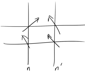
fig. 1. Neighbouring spin cells.

Such a Hamiltonian is left invariant by the transformation \( \BS_n \rightarrow -\BS_n \) since the Hamiltonian is quadratic.

Suppose that \( \phi \rightarrow -\phi\) is a symmetry (it leaves the Lagrangian unchanged). Example

\begin{equation}\label{eqn:qftLecture6:940}
\phi =
\begin{bmatrix}
\phi^1 \\
\phi^2 \\
\vdots
\phi^n \\
\end{bmatrix}
\end{equation}

the Lagrangian
\begin{equation}\label{eqn:qftLecture6:960}
\LL = \inv{2} \partial_\mu \phi^\T \partial^\mu \phi – \frac{m^2}{2} \phi^\T \phi – V(\phi^\T \phi).
\end{equation}
If \( O \) is any \( n \times n \) orthogonal matrix, then it is symmetry since
\begin{equation}\label{eqn:qftLecture6:980}
\phi^\T \phi \rightarrow \phi^\T O^\T O \phi = \phi^\T \phi.
\end{equation}

O(2) model, HW, problem 2. Example for complex \( \phi \)
\begin{equation}\label{eqn:qftLecture6:1000}
\phi \rightarrow e^{i \phi} \phi,
\end{equation}
\begin{equation}\label{eqn:qftLecture6:1020}
\phi = \frac{\psi_1 + i \psi_2}{\sqrt{2}}
\end{equation}

\begin{equation}\label{eqn:qftLecture6:1040}
\begin{bmatrix}
\psi_1 \\
\psi_2
\end{bmatrix}
\rightarrow
\begin{bmatrix}
\cos\alpha & \sin\alpha \\
-\sin\alpha & \cos\alpha
\end{bmatrix}
\begin{bmatrix}
\psi_1 \\
\psi_2
\end{bmatrix}
\end{equation}

PHY2403H Quantum Field Theory. Lecture 5: Klein-Gordon equation, Hamilton’s equations, SHOs, momentum space representation, raising and lowering operators. Taught by Prof. Erich Poppitz

September 25, 2018 phy2403 , , , , , , , , , , ,

[Click here for a PDF of this post with nicer formatting]

Disclaimer

DISCLAIMER: Very rough notes from class. Some additional side notes, but otherwise barely edited.

These are notes for the UofT course PHY2403H, Quantum Field Theory I, taught by Prof. Erich Poppitz fall 2018.

Canonical quantization

Last time we introduced a Lagrangian density associated with the Klein-Gordon equation (with a quadratic potential coupling)
\begin{equation}\label{eqn:qftLecture5:20}
L = \int d^3 x
\lr{
\inv{2} \lr{\partial_0 \phi}^2 – \inv{2} \lr{\spacegrad \phi}^2 – \frac{m^2}{2} \phi^2 – \frac{\lambda}{4} \phi^4
}.
\end{equation}
This Lagrangian density was related to the action by
\begin{equation}\label{eqn:qftLecture5:40}
S = \int dt L = \int dt d^3 x \LL,
\end{equation}
with momentum canonically conjugate to the field \( \phi \) defined as
\begin{equation}\label{eqn:qftLecture5:60}
\Pi(\Bx, t) = \frac{\delta \LL}{\delta \phidot(\Bx, t) } = \PD{\phidot(\Bx, t)}{\LL}
\end{equation}

The Hamiltonian defined as
\begin{equation}\label{eqn:qftLecture5:80}
H = \int d^3 x \lr{ \Pi(\Bx, t) \phidot(\Bx, t) – \LL },
\end{equation}
led to
\begin{equation}\label{eqn:qftLecture5:680}
H
= \int d^3 x
\lr{ \inv{2} \Pi^2 + (\spacegrad \phi)^2 + \inv{2} m^2 \phi^2 + \frac{\lambda}{4} \phi^4 }.
\end{equation}
Like the Lagrangian density, we may introduce a Hamiltonian density \( \mathcal{H} \) as
\begin{equation}\label{eqn:qftLecture5:100}
H = \int d^3 x \mathcal{H}(\Bx, t).
\end{equation}
For our Klein-Gordon system, this is
\begin{equation}\label{eqn:qftLecture5:120}
\mathcal{H}(\Bx, t) =
\inv{2} \Pi^2 + (\spacegrad \phi)^2 + \inv{2} m^2 \phi^2 + \frac{\lambda}{4} \phi^4.
\end{equation}

Canonical Commutation Relations (CCR)

:

We quantize the system by promoting our fields to Heisenberg-Picture (HP) operators, and imposing commutation relations
\begin{equation}\label{eqn:qftLecture5:140}
\antisymmetric{\hat{\Pi}(\Bx, t)}{\hat{\phi}(\By, t)} = -i \delta^3 (\Bx – \By)
\end{equation}

This is in analogy to
\begin{equation}\label{eqn:qftLecture5:160}
\antisymmetric{\hat{p}_i}{\hat{q}_j} = -i \delta_{ij},
\end{equation}

To choose a representation, we may map the \( \Psi \) of QM \( \rightarrow \) to a wave functional \( \Psi[\phi] \)
\begin{equation}\label{eqn:qftLecture5:180}
\hat{\phi}(\By, t) \Psi[\phi] = \phi(\By, t) \Psi[\phi]
\end{equation}

This is similar to the QM wave functions
\begin{equation}\label{eqn:qftLecture5:200}
\begin{aligned}
\hat{q}_i \Psi(\setlr{q}) &= q_i \Psi(q) \\
\hat{p}_i \Psi(\setlr{q}) &= -i \PD{q_i}{} \Psi(p)
\end{aligned}
\end{equation}

Our momentum operator is quantized by expressing it in terms of a variational derivative
\begin{equation}\label{eqn:qftLecture5:220}
\hat{\Pi}(\Bx, t) = -i \frac{\delta}{\delta \phi(\Bx, t)}.
\end{equation}
(Fixme: I’m not really sure exactly what is meant by using the variation derivative \(\delta\) notation here), and to
quantize the Hamiltonian we just add hats, assuming that our fields are all now HP operators
\begin{equation}\label{eqn:qftLecture5:240}
\hat{\mathcal{H}}(\Bx, t)
=
\inv{2} \hat{\Pi}^2 + (\spacegrad \hat{\phi})^2 + \inv{2} m^2 \hat{\phi}^2 + \frac{\lambda}{4} \hat{\phi}^4.
\end{equation}

QM SHO review

Recall the QM SHO had a Hamiltonian
\begin{equation}\label{eqn:qftLecture5:260}
\hat{H} = \inv{2} \hat{p}^2 + \inv{2} \omega^2 \hat{q}^2,
\end{equation}
where
\begin{equation}\label{eqn:qftLecture5:280}
\antisymmetric{\hat{p}}{\hat{q}} = -i,
\end{equation}
and that
HP time evolution operators \( O \) satisfied
\begin{equation}\label{eqn:qftLecture5:700}
\ddt{\hatO} = i \antisymmetric{\hatH}{\hatO}.
\end{equation}
In particular
\begin{equation}\label{eqn:qftLecture5:300}
\begin{aligned}
\ddt{\hat{p}}
&= i \antisymmetric{\hat{H}}{\hatp} \\
&= i \frac{\omega^2}{2} \antisymmetric{\hat{q}^2}{\hatp} \\
&= i \frac{\omega^2}{2} (2 i \hat{q}) \\
&= -i \omega^2 \hat{q},
\end{aligned}
\end{equation}
and
\begin{equation}\label{eqn:qftLecture5:320}
\begin{aligned}
\ddt{\hat{q}}
&= i \antisymmetric{\hat{H}}{\hat{q}} \\
&= i \inv{2} \antisymmetric{\hatp^2}{\hat{q}} \\
&= \frac{i}{2}(-2 i \hatp ) \\
&= \hatp.
\end{aligned}
\end{equation}
Applying the time evolution operator twice, we find
\begin{equation}\label{eqn:qftLecture5:340}
\frac{d^2}{dt^2}{\hat{q}}
= \ddt{\hat{p}}
= – \omega^2 \hat{q}.
\end{equation}
We see that the Heisenberg operators obey the classical equations of motion.

Now we want to try this with the quantized QFT fields we’ve promoted to operators
\begin{equation}\label{eqn:qftLecture5:360}
\begin{aligned}
\ddt{\hat{\Pi}}(\Bx, t)
&= i \antisymmetric{\hatH}{\hat{\Pi}(\Bx, t)} \\
&=
i \int d^3 y \inv{2} \antisymmetric{ \lr{\spacegrad \phihat(\By) }^2 }{\hat{\Pi}(\Bx) }
+
i \int d^3 y \frac{m^2}{2} \antisymmetric{ \phihat(\By)^2 }{\hat{\Pi}(\Bx) }
+
i \frac{\lambda}{4} \int d^3 \antisymmetric{ \phihat(\By)^4 }{\hat{\Pi}(\Bx) }
\end{aligned}
\end{equation}

Starting with the non-gradient commutators, and utilizing the HP field analogues of the relations \( \antisymmetric{\hat{q}^n}{\hatp} = n i \hat{q}^{n-1} \), we find
\begin{equation}\label{eqn:qftLecture5:780}
\int d^3 y \antisymmetric{ \lr{ \phihat(\By) }^2 }{\hat{\Pi}(\Bx) }
=
\int d^3 y 2 i \phihat(\By) \delta^3(\Bx – \By)
= 2 i \phihat(\Bx).
\end{equation}
\begin{equation}\label{eqn:qftLecture5:740}
\int d^3 y \antisymmetric{ \lr{ \phihat(\By) }^4 }{\hat{\Pi}(\Bx) }
=
\int d^3 y 4 i \phihat(\By)^3 \delta^3(\Bx – \By)
= 4 i \phihat(\Bx)^3.
\end{equation}
For the gradient commutators, we have more work. Prof Poppitz blitzed through that, just calling it integration by parts. I had trouble seeing what he was doing, so here’s a more explicit dumb expansion required to calculate the commutator
\begin{equation}\label{eqn:qftLecture5:720}
\begin{aligned}
\int d^3 y (\spacegrad \phihat(\By))^2 \hat{\Pi}(\Bx)
&=
\int d^3 y
\lr{ \spacegrad \phihat(\By) \cdot \spacegrad \phihat(\By) } \hat{\Pi}(\Bx) \\
&=
\int d^3 y
\spacegrad \phihat(\By) \cdot
\lr{ \spacegrad (\phihat(\By) \hat{\Pi}(\Bx)) } \\
&=
\int d^3 y
\spacegrad \phihat(\By) \cdot
\lr{ \spacegrad (\hat{\Pi}(\Bx) \phihat(\By) + i \delta^3(\Bx – \By)) } \\
&=
\int d^3 y
\Biglr{
\spacegrad \lr{ \phihat(\By) \hat{\Pi}(\Bx) } \cdot \spacegrad \phihat(\By)
+ i
\spacegrad \phihat(\By) \cdot \spacegrad \delta^3(\Bx – \By)
} \\
&=
\int d^3 y
\Biglr{
\spacegrad \lr{ \hat{\Pi}(\Bx) \phihat(\By) + i \delta^3(\Bx – \By) } \cdot \spacegrad \phihat(\By)
+ i
\spacegrad \phihat(\By) \cdot \spacegrad \delta^3(\Bx – \By)
} \\
&=
\int d^3 y
\hat{\Pi}(\Bx)
\lr{
\spacegrad \phihat(\By) \cdot \spacegrad \phihat(\By)
}
+ 2 i
\int d^3 y
\spacegrad \phihat(\By) \cdot \spacegrad \delta^3(\Bx – \By) \\
&=
\int d^3 y
\hat{\Pi}(\Bx) \spacegrad^2 \phihat(\By)
+
2 i
\int d^3 y
\spacegrad \cdot \lr{ \delta^3(\Bx – \By) \spacegrad \phihat(\By) }

2 i
\int d^3 y
\delta^3(\Bx – \By) \spacegrad^2 \phihat(\By) \\
&=
\int d^3 y
\hat{\Pi}(\Bx) \spacegrad^2 \phihat(\By)
+
2 i
\int_\partial d^2 y
\delta^3(\Bx – \By)
\ncap \cdot \spacegrad \phihat(\By)

2 i \spacegrad^2 \phihat(\Bx).
\end{aligned}
\end{equation}
Here we take advantage of the fact that the derivative operators \( \spacegrad = \spacegrad_\By \) commute with \( \hat{\Pi}(\Bx) \), and use the identity
\( \spacegrad \cdot (a \spacegrad b) = (\spacegrad a) \cdot (\spacegrad b) + a \spacegrad^2 b \), so the commutator is
\begin{equation}\label{eqn:qftLecture5:800}
\begin{aligned}
\int d^3 y \antisymmetric{(\spacegrad \phihat(\By))^2}{\hat{\Pi}(\Bx)}
&=
2 i
\int_\partial d^2 y
\delta^3(\Bx – \By)
\ncap \cdot \spacegrad \phihat(\By)

2 i \spacegrad^2 \phihat(\Bx) \\
&=

2 i \spacegrad^2 \phihat(\Bx),
\end{aligned}
\end{equation}
where the boundary integral is presumed to be zero (without enough justification.) All the pieces can now be put back together
\begin{equation}\label{eqn:qftLecture5:820}
\ddt{} \hat{\Pi}(\Bx, t)
=
\spacegrad^2 \phihat(\Bx, t)

m^2 \phihat(\Bx, t)

\lambda \phihat^3(\Bx, t).
\end{equation}

Now, for the \( \phihat \) time evolution, which is much easier
\begin{equation}\label{eqn:qftLecture5:380}
\begin{aligned}
\ddt{\hat{\phi}}(\Bx, t)
&= i \antisymmetric{\hatH}{\hat{\phi}(\Bx, t)} \\
&= i \inv{2} \int d^3 y \antisymmetric{\hat{\Pi}^2(\By)}{\hat{\phi}(\Bx)} \\
&= i \inv{2} \int d^3 y (-2 i) \hat{\Pi}(\By, t) \delta^3(\Bx – \By) \\
&= \hat{\Pi}(\Bx, t)
\end{aligned}
\end{equation}
\begin{equation}\label{eqn:qftLecture5:400}
\frac{d^2}{dt^2}{\hat{\phi}}(\Bx, t)
=
\spacegrad^2 \phi
-m^2 \phi – \lambda \phihat^3.
\end{equation}
That is
\begin{equation}\label{eqn:qftLecture5:420}
\ddot{\phihat} – \spacegrad^2 \phihat + m^2 \phihat + \lambda \phihat^3 = 0,
\end{equation}
which is the classical Euler-Lagrange equation, also obeyed by the Heisenberg operator \( \phi(\Bx, t) \). When \( \lambda = 0 \) this is the Klein-Gordon equation.

Momentum space representation.

Dropping hats, we now consider the momentum space representation of our operators, as determined by Fourier transform pairs
\begin{equation}\label{eqn:qftLecture5:440}
\begin{aligned}
\phi(\Bx, t) &= \int \frac{d^3 p}{(2\pi)^3} e^{i \Bp \cdot \Bx} \tilde{\phi}(\Bp, t) \\
\tilde{\phi}(\Bp, t) &= \int d^3 x e^{-i \Bp \cdot \Bx} \phi(\Bx, t)
\end{aligned}
\end{equation}

We can discover a representation of the delta function by applying these both in turn
\begin{equation}\label{eqn:qftLecture5:480}
\tilde{\phi}(\Bp, t)
= \int d^3 x e^{-i \Bp \cdot \Bx} \int \frac{d^3 q}{(2 \pi)^3} e^{i \Bq \cdot \Bx} \tilde{\phi}(\Bq, t)
\end{equation}
so
\begin{equation}\label{eqn:qftLecture5:500}
\boxed{
\int d^3 x e^{i \BA \cdot \Bx} = (2 \pi)^3 \delta^3(\BA)
}
\end{equation}

Also observe that \( \phi^\conj(\Bx, t) = \phi(\Bx, t) \) iff \( \tilde{\phi}(\Bp, t) = \tilde{\phi}^\conj(-\Bp, t) \).

We want the EOM for \( \tilde{\phi}(\Bp, t) \) where the operator obeys the KG equation
\begin{equation}\label{eqn:qftLecture5:520}
\lr{ \partial_t^2 – \spacegrad^2 + m^2 } \phi(\Bx, t) = 0
\end{equation}

Inserting the transform relation \ref{eqn:qftLecture5:440} we get
\begin{equation}\label{eqn:qftLecture5:540}
\int \frac{d^3 p}{(2 \pi)^3} e^{i \Bp \cdot \Bx}
\lr{
\ddot{\tilde{\phi}}(\Bp, t) + \lr{ \Bp^2 + m^2 }
\tilde{\phi}(\Bp, t)
}
= 0,
\end{equation}
or
\begin{equation}\label{eqn:qftLecture5:580}
\boxed{
\ddot{\tilde{\phi}}(\Bp, t) = – \omega_\Bp^2 \,\tilde{\phi}(\Bp, t),
}
\end{equation}
where
\begin{equation}\label{eqn:qftLecture5:560}
\omega_\Bp = \sqrt{ \Bp^2 + m^2 }.
\end{equation}
The Fourier components of the HP operators are SHOs!

As we have SHO’s and know how to deal with these in QM, we use the same strategy, introducing raising and lowering operators
\begin{equation}\label{eqn:qftLecture5:600}
\tilde{\phi}(\Bp, t) = \inv{\sqrt{2 \omega_\Bp}} \lr{ e^{-i \omega_\Bp t } a_\Bp + e^{i \omega_\Bp t} a^\dagger_{-\Bp}
}
\end{equation}

Observe that
\begin{equation}\label{eqn:qftLecture5:840}
\begin{aligned}
\tilde{\phi}^\dagger(-\Bp, t)
&= \inv{\sqrt{2 \omega_\Bp}} \lr{ e^{i \omega_\Bp t } a^\dagger_{-\Bp} + e^{-i \omega_\Bp t} a_{\Bp} } \\
&=
\tilde{\phi}(\Bp, t),
\end{aligned}
\end{equation}
or
\begin{equation}\label{eqn:qftLecture5:620}
\tilde{\phi}^\dagger(\Bp, t) = \tilde{\phi}(-\Bp, t),
\end{equation}
so \( \phi(\Bp, t) \) has a real representation in terms of \( a_\Bp \).

We will find (Wednesday) that
\begin{equation}\label{eqn:qftLecture5:640}
\antisymmetric{a_\Bq}{a^+_\Bp} = \delta^3(\Bp – \Bq) (2 \pi)^3.
\end{equation}

These are equivalent to
\begin{equation}\label{eqn:qftLecture5:660}
\antisymmetric{\hat{\Pi}(\By, t)}{\tilde{\phi}(\Bx, t)} = -i \delta^3(\Bx – \By)
\end{equation}