[Click here for a PDF of this post with nicer formatting]
Disclaimer
Peeter’s lecture notes from class. These may be incoherent and rough.
These are notes for the UofT course PHY1520, Graduate Quantum Mechanics, taught by Prof. Paramekanti, covering [1] ch. 5 content.
Another approach (for last time?)
Imagine we perturb a potential, say a harmonic oscillator with an electric field
\begin{equation}\label{eqn:qmLecture22:20}
V_0(x) = \inv{2} k x^2
\end{equation}
\begin{equation}\label{eqn:qmLecture22:40}
V(x) = \mathcal{E} e x
\end{equation}
After minimizing the energy, using \( \PDi{x}{V} = 0 \), we get
\begin{equation}\label{eqn:qmLecture22:60}
\inv{2} k x^2 + \mathcal{E} e x \rightarrow k x^\conj = – e \mathcal{E}
\end{equation}
\begin{equation}\label{eqn:qmLecture22:80}
p^\conj = -e x^\conj = – \frac{e^2 \mathcal{E}}{k}
\end{equation}
For such a system the polarizability is
\begin{equation}\label{eqn:qmLecture22:100}
\alpha = \frac{e^2 }{k}
\end{equation}
\begin{equation}\label{eqn:qmLecture22:120}
\begin{aligned}
\inv{2} k \lr{ -\frac{ e \mathcal{E}}{k} }^2 + \mathcal{E} e \lr{ – \frac{e \mathcal{E}}{k} }
&= – \inv{2} \lr{ \frac{e^2}{k} } \mathcal{E}^2 \\
&= – \inv{2} \alpha \mathcal{E}^2
\end{aligned}
\end{equation}
Van der Wall potential
\begin{equation}\label{eqn:qmLecture22:140}
H_0 =
H_{0 1} + H_{0 2},
\end{equation}
where
\begin{equation}\label{eqn:qmLecture22:160}
H_{0 \alpha} = \frac{p_\alpha^2}{2m} – \frac{e^2}{4 \pi \epsilon_0 \Abs{ \Br_\alpha – \BR_\alpha} }, \qquad \alpha = 1,2
\end{equation}
The full interaction potential is
\begin{equation}\label{eqn:qmLecture22:180}
V =
\frac{e^2}{4 \pi \epsilon_0} \lr{
\inv{\Abs{\BR_1 – \BR_2}}
+
\inv{\Abs{\Br_1 – \Br_2}}
–
\inv{\Abs{\Br_1 – \BR_2}}
–
\inv{\Abs{\Br_2 – \BR_1}}
}
\end{equation}
Let
\begin{equation}\label{eqn:qmLecture22:200}
\Bx_\alpha = \Br_\alpha – \BR_\alpha,
\end{equation}
\begin{equation}\label{eqn:qmLecture22:220}
\BR = \BR_1 – \BR_2,
\end{equation}
as sketched in fig. 1.
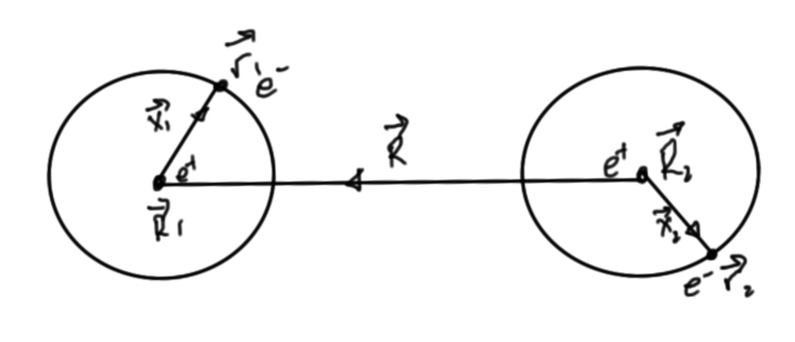
fig. 1. Two atom interaction.
\begin{equation}\label{eqn:qmLecture22:240}
H_{0 \alpha}
=
\frac{\Bp^2}{2m}
-\frac{e^2}{4 \pi \epsilon_0 \Abs{\Bx_\alpha}}
\end{equation}
which allows the total interaction potential to be written
\begin{equation}\label{eqn:qmLecture22:260}
V =
\frac{e^2}{4 \pi \epsilon_0 R}
\lr{
1
+
\frac{R}{\Abs{\Bx_1 – \Bx_2 + \BR}}
–
\frac{R}{\Abs{\Bx_1 + \BR}}
–
\frac{R}{\Abs{-\Bx_2 + \BR}}
}
\end{equation}
For \( R \gg x_1, x_2 \), this interaction potential, after a multipole expansion, is approximately
\begin{equation}\label{eqn:qmLecture22:280}
V =
\frac{e^2}{4 \pi \epsilon_0} \lr{
\frac{\Bx_1 \cdot \Bx_2}{\Abs{\BR}^3}
-3 \frac{
(\Bx_1 \cdot \BR)
(\Bx_2 \cdot \BR)
}{\Abs{\BR}^5}
}
\end{equation}
1. \( O(\lambda) \)
.
With
\begin{equation}\label{eqn:qmLecture22:300}
\psi_0 = \ket{ 1s, 1s }
\end{equation}
\begin{equation}\label{eqn:qmLecture22:320}
\Delta E^{(1)} = \bra{\psi_0} V \ket{\psi_0}
\end{equation}
The two particle wave functions are of the form
\begin{equation}\label{eqn:qmLecture22:340}
\braket{ \Bx_1, \Bx_2 }{\psi_0} =
\psi_{1s}(\Bx_1)
\psi_{1s}(\Bx_2),
\end{equation}
so braket integrals must be evaluated over a six-fold space. Recall that
\begin{equation}\label{eqn:qmLecture22:740}
\psi_{1s} = \inv{\sqrt{\pi} a_0^{3/2} } e^{-r/a_0},
\end{equation}
so
\begin{equation}\label{eqn:qmLecture22:760}
\bra{\psi_{1s}} x_i \ket{\psi_{1s}}
\propto
\int_0^\pi \sin\theta d\theta \int_0^{2\pi} d\phi x_i
\end{equation}
where
\begin{equation}\label{eqn:qmLecture22:780}
x_i \in \setlr{ r \sin\theta \cos\phi, r \sin\theta \sin\phi, r \cos\theta }.
\end{equation}
The \( x, y \) integrals are zero because of the \( \phi \) integral, and the \( z \) integral is proportional to \( \int_0^\pi \sin(2 \theta) d\theta \), which is also zero. This leads to zero averages
\begin{equation}\label{eqn:qmLecture22:360}
\expectation{\Bx_1} = 0 = \expectation{\Bx_2}
\end{equation}
so
\begin{equation}\label{eqn:qmLecture22:380}
\Delta E^{(1)} = 0.
\end{equation}
2. \( O(\lambda^2) \)
.
\begin{equation}\label{eqn:qmLecture22:400}
\begin{aligned}
\Delta E^{(2)}
&= \sum_{n \ne 0} \frac{ \Abs{ \bra{\psi_n } V \ket{\psi_0} }^2 }{E_0 – E_n} \\
&= \sum_{n \ne 0} \frac{ \bra{\psi_0 } V \ket{\psi_n} \bra{\psi_n } V \ket{\psi_0} }{E_0 – E_n}.
\end{aligned}
\end{equation}
This is a sum over all excited states. We expect that this will be of the form
\begin{equation}\label{eqn:qmLecture22:420}
\Delta E^{(2)} = – \lr{ \frac{e^2}{4 \pi \epsilon_0} }^2 \frac{C_6}{R^6}
\end{equation}
\( \Bx_1 \) and \( \Bx_2 \) are dipole operators. The first time this has a non-zero expectation is when we go from the 1s to the 2p states (both 1s and 2s states are spherically symmetric).
Noting that \( E_n = -e^2/2 n^2 a_0 \), we can compute a minimum bound for the energy denominator
\begin{equation}\label{eqn:qmLecture22:440}
\begin{aligned}
\lr{E_n – E_0}^{\mathrm{min}}
&= 2 \lr{ E_{2p} – E_{1s} } \\
&= 2 E_{1s} \lr{ \inv{4} – 1 } \\
&= 2 \frac{3}{4} \Abs{E_{1s}} \\
&= \frac{3}{2} \Abs{E_{1s}}.
\end{aligned}
\end{equation}
Note that the factor of two above comes from summing over the energies for both electrons. This gives us
\begin{equation}\label{eqn:qmLecture22:460}
C_6
=
\frac{3}{2} \Abs{E_{1s}}
\bra{\psi_0 } \tilde{V} \ket{\psi_0},
\end{equation}
where
\begin{equation}\label{eqn:qmLecture22:480}
\tilde{V} =
\lr{
\Bx_1 \cdot \Bx_2
-3
(\Bx_1 \cdot \Rcap)
(\Bx_2 \cdot \Rcap)
}
\end{equation}
What about degeneracy?
\begin{equation}\label{eqn:qmLecture22:500}
\Delta E^{(2)}_n
= \sum_{m \ne n} \frac{ \Abs{ \bra{\psi_n } V \ket{\psi_0} }^2 }{E_0 – E_n}
\end{equation}
If \( \bra{\psi_n} V \ket{\psi_m} \propto \delta_{n m} \) then it’s okay.
In general the we can’t expect the matrix element will be anything but fully populated, say
\begin{equation}\label{eqn:qmLecture22:520}
V =
\begin{bmatrix}
V_{11} & V_{12} & V_{13} & V_{14} \\
V_{21} & V_{22} & V_{23} & V_{24} \\
V_{31} & V_{32} & V_{33} & V_{34} \\
V_{41} & V_{42} & V_{43} & V_{44} \\
\end{bmatrix},
\end{equation}
If we choose a basis so that
\begin{equation}\label{eqn:qmLecture22:540}
V =
\begin{bmatrix}
V_{11} & & & \\
& V_{22} & & \\
& & V_{33} & \\
& & & V_{44} \\
\end{bmatrix}.
\end{equation}
When this is the case, we have no mixing of elements in the sum of \ref{eqn:qmLecture22:500}
Degeneracy in the Stark effect
\begin{equation}\label{eqn:qmLecture22:560}
H = H_0 + e \mathcal{E} z,
\end{equation}
where
\begin{equation}\label{eqn:qmLecture22:580}
H_0 = \frac{\Bp^2}{2m} – \frac{e}{4 \pi \epsilon_0} \inv{\Abs{\Bx}}
\end{equation}
Consider the states \( 2s, 2 p_x, 2p_y, 2p_z \), for which \( E_n^{(0)} \equiv E_{2 s} \), as sketched in fig. 2.
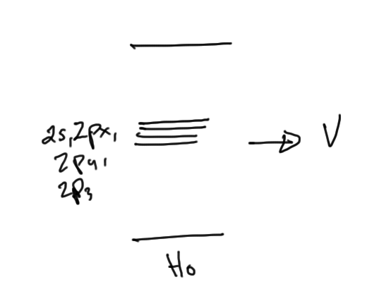
fig. 2. 2s 2p degeneracy.
Because of spherical symmetry
\begin{equation}\label{eqn:qmLecture22:600}
\begin{aligned}
\bra{2 s} e \mathcal{E} z \ket{ 2 s} &= 0 \\
\bra{2 p_x} e \mathcal{E} z \ket{ 2 p_x} &= 0 \\
\bra{2 p_y} e \mathcal{E} z \ket{ 2 p_y} &= 0 \\
\bra{2 p_z} e \mathcal{E} z \ket{ 2 p_z} &= 0 \\
\end{aligned}
\end{equation}
Looking at odd and even properties, it turns out that the only off-diagonal matrix element is
\begin{equation}\label{eqn:qmLecture22:620}
\bra{2 s} e \mathcal{E} z \ket{ 2 p_z } = V_1 = -3 e \mathcal{E} a_0.
\end{equation}
With a \( \setlr{ 2s, 2p_x, 2p_y, 2p_z } \) basis the potential matrix is
\begin{equation}\label{eqn:qmLecture22:640}
\begin{bmatrix}
0 & 0 & 0 & V_1 \\
0 & 0 & 0 & 0 \\
0 & 0 & 0 & 0 \\
V_1^\conj & 0 & 0 & 0 \\
\end{bmatrix}
\end{equation}
\begin{equation}\label{eqn:qmLecture22:660}
\begin{bmatrix}
0 & -\Abs{V_1} \\
-\Abs{V_1} & 0 \\
\end{bmatrix}
\end{equation}
implies that the energy splitting goes as
\begin{equation}\label{eqn:qmLecture22:680}
E_{2s} \rightarrow
E_{2s} \pm \Abs{V_1},
\end{equation}
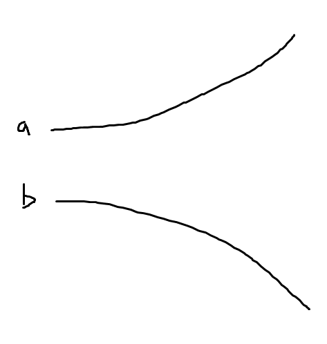
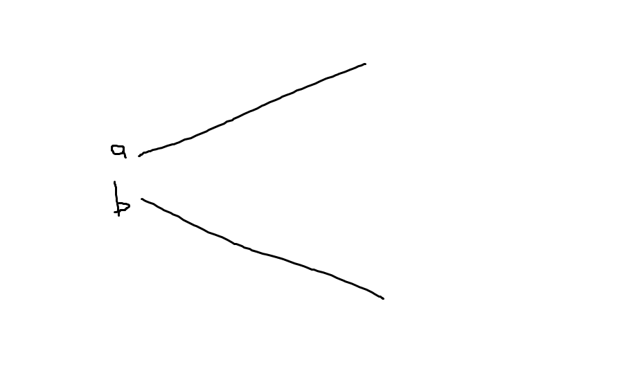
as sketched in fig. 3.
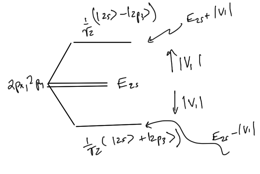
fig. 3. Stark effect energy level splitting.
The diagonalizing states corresponding to eigenvalues \( \pm 3 a_0 \mathcal{E} \), are \( (\ket{2s} \mp \ket{2p_z})/\sqrt{2} \).
The matrix element above is calculated explicitly in lecture22Integrals.nb.
The degeneracy that is left unsplit here, and has to be accounted for should we attempt higher order perturbation calculations.
Appendix. Multipole expansion
Noting that
\begin{equation}\label{eqn:qmLecture22:700}
\begin{aligned}
\lr{1 + \epsilon}^{-1/2}
&=
1 -\inv{2} \epsilon -\inv{2}\lr{\frac{-3}{2}}\inv{2!} \epsilon^2 \\
&=
1 -\inv{2} \epsilon + \frac{3}{8} \epsilon^2,
\end{aligned}
\end{equation}
we have
\begin{equation}\label{eqn:qmLecture22:720}
\begin{aligned}
\frac{R}{\Abs{\Bepsilon + \BR}}
&=
\frac{1}{\Abs{\frac{\Bepsilon}{R} + \Rcap}} \\
&=
\lr{ 1 + 2 \frac{\Bepsilon}{R} \cdot \Rcap + \lr{\frac{\Bepsilon}{R}}^2 }^{-1/2} \\
&=
1 – \frac{\Bepsilon}{R} \cdot \Rcap -\inv{2} \lr{\frac{\Bepsilon}{R}}^2
+ \frac{3}{8}
\lr{ 2 \frac{\Bepsilon}{R} \cdot \Rcap + \lr{\frac{\Bepsilon}{R}}^2 }^2 \\
&=
1 – \frac{\Bepsilon}{R} \cdot \Rcap -\inv{2} \lr{\frac{\Bepsilon}{R}}^2
+ \frac{3}{8}
\lr{ 4 \lr{ \frac{\Bepsilon}{R} \cdot \Rcap}^2 + \lr{\frac{\Bepsilon}{R}}^4
+ 4 \frac{\Bepsilon}{R} \cdot \Rcap \lr{\frac{\Bepsilon}{R}}^2
} \\
&\approx
1 – \frac{\Bepsilon}{R} \cdot \Rcap -\inv{2} \lr{\frac{\Bepsilon}{R}}^2
+ \frac{3}{2}
\lr{ \frac{\Bepsilon}{R} \cdot \Rcap}^2 .
\end{aligned}
\end{equation}
Inserting the values from the brackets of \ref{eqn:qmLecture22:260} we have
\begin{equation}\label{eqn:qmLecture22:800}
\begin{aligned}
1
+
\frac{R}{\Abs{\Bx_1 – \Bx_2 + \BR}}
&-
\frac{R}{\Abs{\Bx_1 + \BR}}
–
\frac{R}{\Abs{-\Bx_2 + \BR}} \\
&=
– \frac{\lr{ \Bx_1 – \Bx_2 }}{R} \cdot \Rcap -\inv{2} \lr{\frac{\lr{ \Bx_1 – \Bx_2 }}{R}}^2
+ \frac{3}{2}
\lr{ \frac{\lr{ \Bx_1 – \Bx_2 }}{R} \cdot \Rcap}^2 \\
&\quad + \frac{\Bx_1}{R} \cdot \Rcap +\inv{2} \lr{\frac{\Bx_1}{R}}^2
– \frac{3}{2}
\lr{ \frac{\Bx_1}{R} \cdot \Rcap}^2 \\
&\quad – \frac{\Bx_2}{R} \cdot \Rcap +\inv{2} \lr{\frac{\Bx_2}{R}}^2
– \frac{3}{2}
\lr{ \frac{\Bx_2}{R} \cdot \Rcap}^2 \\
&=
\frac{\Bx_1}{R} \cdot \frac{\Bx_2 }{R}
+ \frac{3}{2}
\lr{ \frac{\lr{ \Bx_1 – \Bx_2 }}{R} \cdot \Rcap}^2 \\
&\quad
– \frac{3}{2}
\lr{ \frac{\Bx_1}{R} \cdot \Rcap}^2 \\
&\quad
– \frac{3}{2}
\lr{ \frac{\Bx_2}{R} \cdot \Rcap}^2 \\
&=
\frac{\Bx_1}{R} \cdot \frac{\Bx_2 }{R}
– 3 \frac{\Bx_1}{R} \cdot \Rcap \frac{\Bx_2}{R} \cdot \Rcap.
\end{aligned}
\end{equation}
This proves \ref{eqn:qmLecture22:280}.
References
[1] Jun John Sakurai and Jim J Napolitano. Modern quantum mechanics. Pearson Higher Ed, 2014.