interaction picture

PHY2403H Quantum Field Theory. Lecture 14: Time evolution, Hamiltonian perturbation, ground state. Taught by Prof. Erich Poppitz

October 29, 2018 phy2403 , , , , , ,

[Click here for a PDF of this post with nicer formatting]

DISCLAIMER: Very rough notes from class, with some additional side notes.

These are notes for the UofT course PHY2403H, Quantum Field Theory, taught by Prof. Erich Poppitz, fall 2018.

Review

Given a field \( \phi(t_0, \Bx) \), satisfying the commutation relations
\begin{equation}\label{eqn:qftLecture14:20}
\antisymmetric{\pi(t_0, \Bx)}{\phi(t_0, \By)} = -i \delta(\Bx – \By)
\end{equation}
we introduced an interaction picture field given by
\begin{equation}\label{eqn:qftLecture14:40}
\phi_I(t, x) = e^{i H_0(t- t_0)} \phi(t_0, \Bx) e^{-iH_0(t – t_0)}
\end{equation}
related to the Heisenberg picture representation by
\begin{equation}\label{eqn:qftLecture14:60}
\phi_H(t, x)
= e^{i H(t- t_0)} \phi(t_0, \Bx) e^{-iH(t – t_0)}
= U^\dagger(t, t_0) \phi_I(t, \Bx) U(t, t_0),
\end{equation}
where \( U(t, t_0) \) is the time evolution operator.
\begin{equation}\label{eqn:qftLecture14:80}
U(t, t_0) =
e^{i H_0(t – t_0)}
e^{-i H(t – t_0)}
\end{equation}
We argued that
\begin{equation}\label{eqn:qftLecture14:100}
i \PD{t}{} U(t, t_0) = H_{\text{I,int}}(t) U(t, t_0)
\end{equation}
We found the glorious expression
\begin{equation}\label{eqn:qftLecture14:120}
\boxed{
\begin{aligned}
U(t, t_0)
&= T \exp{\lr{ -i \int_{t_0}^t H_{\text{I,int}}(t’) dt’}} \\
&=
\sum_{n = 0}^\infty \frac{(-i)^n}{n!} \int_{t_0}^t dt_1 dt_2 \cdots dt_n T\lr{ H_{\text{I,int}}(t_1) H_{\text{I,int}}(t_2) \cdots H_{\text{I,int}}(t_n) }
\end{aligned}
}
\end{equation}

However, what we are really after is
\begin{equation}\label{eqn:qftLecture14:140}
\bra{\Omega} T(\phi(x_1) \cdots \phi(x_n)) \ket{\Omega}
\end{equation}
Such a product has many labels and names, and we’ll describe it as “vacuum expectation values of time-ordered products of arbitrary #’s of local Heisenberg operators”.

Perturbation

Following section 4.2, [1].

\begin{equation}\label{eqn:qftLecture14:160}
\begin{aligned}
H &= \text{exact Hamiltonian} = H_0 + H_{\text{int}}
\\
H_0 &= \text{free Hamiltonian.
}
\end{aligned}
\end{equation}
We know all about \( H_0 \) and assume that it has a lowest (ground state) \( \ket{0} \), the “vacuum” state of \( H_0 \).

\( H \) has eigenstates, in particular \( H \) is assumed to have a unique ground state \( \ket{\Omega} \) satisfying
\begin{equation}\label{eqn:qftLecture14:180}
H \ket{\Omega} = \ket{\Omega} E_0,
\end{equation}
and has states \( \ket{n} \), representing excited (non-vacuum states with energies > \( E_0 \)).
These states are assumed to be a complete basis
\begin{equation}\label{eqn:qftLecture14:200}
\mathbf{1} = \ket{\Omega}\bra{\Omega} + \sum_n \ket{n}\bra{n} + \int dn \ket{n}\bra{n}.
\end{equation}
The latter terms may be written with a superimposed sum-integral notation as
\begin{equation}\label{eqn:qftLecture14:440}
\sum_n + \int dn
=
{\int\kern-1em\sum}_n,
\end{equation}
so the identity operator takes the more compact form
\begin{equation}\label{eqn:qftLecture14:460}
\mathbf{1} = \ket{\Omega}\bra{\Omega} + {\int\kern-1em\sum}_n \ket{n}\bra{n}.
\end{equation}

For some time \( T \) we have
\begin{equation}\label{eqn:qftLecture14:220}
e^{-i H T} \ket{0} = e^{-i H T}
\lr{
\ket{\Omega}\braket{\Omega}{0} + {\int\kern-1em\sum}_n \ket{n}\braket{n}{0}
}.
\end{equation}

We now wish to argue that the \( {\int\kern-1em\sum}_n \) term can be ignored.

Argument 1:

This is something of a fast one, but one can consider a formal transformation \( T \rightarrow T(1 – i \epsilon) \), where \( \epsilon \rightarrow 0^+ \), and consider very large \( T \). This gives
\begin{equation}\label{eqn:qftLecture14:240}
\begin{aligned}
\lim_{T \rightarrow \infty, \epsilon \rightarrow 0^+}
e^{-i H T(1 – i \epsilon)} \ket{0}
&=
\lim_{T \rightarrow \infty, \epsilon \rightarrow 0^+}
e^{-i H T(1 – i \epsilon)}
\lr{
\ket{\Omega}\braket{\Omega}{0} + {\int\kern-1em\sum}_n \ket{n}\braket{n}{0}
} \\
&=
\lim_{T \rightarrow \infty, \epsilon \rightarrow 0^+}
e^{-i E_0 T – E_0 \epsilon T}
\ket{\Omega}\braket{\Omega}{0} + {\int\kern-1em\sum}_n e^{-i E_n T – \epsilon E_n T} \ket{n}\braket{n}{0} \\
&=
\lim_{T \rightarrow \infty, \epsilon \rightarrow 0^+}
e^{-i E_0 T – E_0 \epsilon T}
\lr{
\ket{\Omega}\braket{\Omega}{0} + {\int\kern-1em\sum}_n e^{-i (E_n -E_0) T – \epsilon T (E_n – E_0)} \ket{n}\braket{n}{0}
}
\end{aligned}
\end{equation}
The limits are evaluated by first taking \( T \) to infinity, then only after that take \( \epsilon \rightarrow 0^+ \). Doing this, the sum is dominated by the ground state contribution, since each excited state also has a \( e^{-\epsilon T(E_n – E_0)} \) suppression factor (in addition to the leading suppression factor).

Argument 2:

With the hand waving required for the argument above, it’s worth pointing other (less formal) ways to arrive at the same result. We can write
\begin{equation}\label{eqn:qftLecture14:260}
sectionumInt \ket{n}\bra{n} \rightarrow
\sum_k \int \frac{d^3 p}{(2 \pi)^3} \ket{\Bp, k}\bra{\Bp, k}
\end{equation}
where \( k \) is some unknown quantity that we are summing over.
If we have
\begin{equation}\label{eqn:qftLecture14:280}
H \ket{\Bp, k} = E_{\Bp, k} \ket{\Bp, k},
\end{equation}
then
\begin{equation}\label{eqn:qftLecture14:300}
e^{-i H T} sectionumInt \ket{n}\bra{n}
=
\sum_k \int \frac{d^3 p}{(2 \pi)^3} \ket{\Bp, k} e^{-i E_{\Bp, k}} \bra{\Bp, k}.
\end{equation}
If we take matrix elements
\begin{equation}\label{eqn:qftLecture14:320}
\begin{aligned}
\bra{A}
e^{-i H T} sectionumInt \ket{n}\bra{n} \ket{B}
&=
\sum_k \int \frac{d^3 p}{(2 \pi)^3} \braket{A}{\Bp, k} e^{-i E_{\Bp, k}} \braket{\Bp, k}{B} \\
&=
\sum_k \int \frac{d^3 p}{(2 \pi)^3} e^{-i E_{\Bp, k}} f(\Bp).
\end{aligned}
\end{equation}
If we assume that \( f(\Bp) \) is a well behaved smooth function, we have “infinite” frequency oscillation within the envelope provided by the amplitude of that function, as depicted in fig. 1.
The Riemann-Lebesgue lemma [2] describes such integrals, the result of which is that such an integral goes to zero. This is a different sort of hand waving argument, but either way, we can argue that only the ground state contributes to the sum \ref{eqn:qftLecture14:220} above.

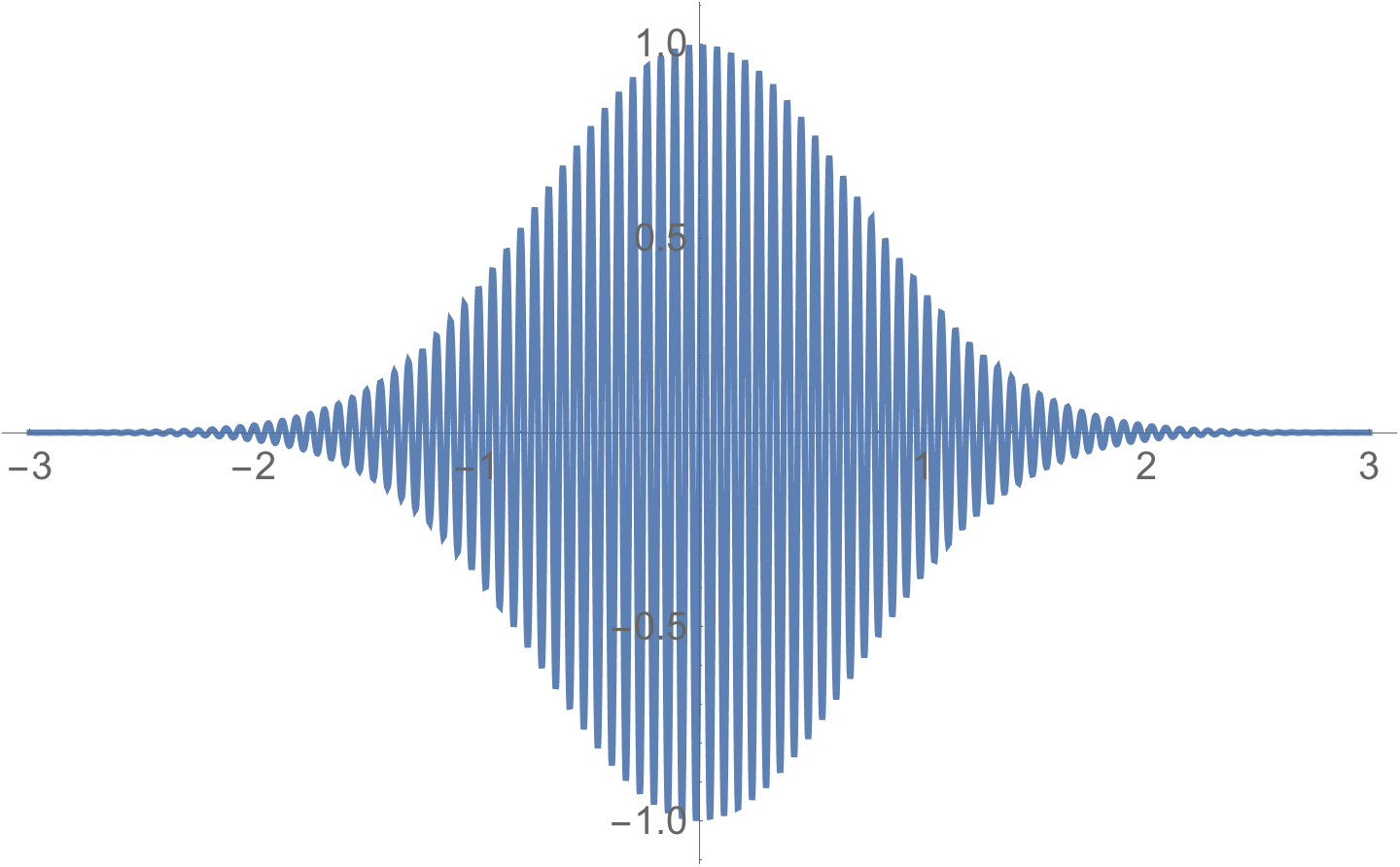
fig. 1. High frequency oscillations within envelope of well behaved function.


Ground state of the perturbed Hamiltonian.

With the excited states ignored, we are left with
\begin{equation}\label{eqn:qftLecture14:340}
e^{-i H T} \ket{0} = e^{-i E_0 T} \ket{\Omega}\braket{\Omega}{0}
\end{equation}
in the \( T \rightarrow \infty(1 – i \epsilon) \) limit. We can now write the ground state as

\begin{equation}\label{eqn:qftLecture14:360}
\begin{aligned}
\ket{\Omega}
&=
\evalbar{
\frac{ e^{i E_0 T – i H T } \ket{0} }{
\braket{\Omega}{0}
}
}{ T \rightarrow \infty(1 – i \epsilon) } \\
&=
\evalbar{
\frac{ e^{- i H T } \ket{0} }{
e^{-i E_0 T} \braket{\Omega}{0}
}
}{ T \rightarrow \infty(1 – i \epsilon) }.
\end{aligned}
\end{equation}
Shifting the very large \( T \rightarrow T + t_0 \) shouldn’t change things, so
\begin{equation}\label{eqn:qftLecture14:480}
\ket{\Omega}
=
\evalbar{
\frac{ e^{- i H (T + t_0) } \ket{0} }{
e^{-i E_0 (T + t_0) } \braket{\Omega}{0}
}
}{ T \rightarrow \infty(1 – i \epsilon) }.
\end{equation}

A bit of manipulation shows that the operator in the numerator has the structure of a time evolution operator.

Claim: (DIY):

\Cref{eqn:qftLecture14:80}, \ref{eqn:qftLecture14:120} may be generalized to
\begin{equation}\label{eqn:qftLecture14:400}
U(t, t’) = e^{i H_0(t – t_0)} e^{-i H(t – t’)} e^{-i H_0(t’ – t_0)} =
T \exp{\lr{ -i \int_{t’}^t H_{\text{I,int}}(t”) dt”}}.
\end{equation}
Observe that we recover \ref{eqn:qftLecture14:120} when \( t’ = t_0 \).  Using \ref{eqn:qftLecture14:400} we find
\begin{equation}\label{eqn:qftLecture14:520}
\begin{aligned}
U(t_0, -T) \ket{0}
&= e^{i H_0(t_0 – t_0)} e^{-i H(t_0 + T)} e^{-i H_0(-T – t_0)} \ket{0} \\
&= e^{-i H(t_0 + T)} e^{-i H_0(-T – t_0)} \ket{0} \\
&= e^{-i H(t_0 + T)} \ket{0},
\end{aligned}
\end{equation}
where we use the fact that \( e^{i H_0 \tau} \ket{0} = \lr{ 1 + i H_0 \tau + \cdots } \ket{0} = 1 \ket{0}, \) since \( H_0 \ket{0} = 0 \).

We are left with
\begin{equation}\label{eqn:qftLecture14:420}
\boxed{
\ket{\Omega}
= \frac{U(t_0, -T) \ket{0} }{e^{-i E_0(t_0 – (-T))} \braket{\Omega}{0}}.
}
\end{equation}

We are close to where we want to be. Wednesday we finish off, and then start scattering and Feynman diagrams.

References

[1] Michael E Peskin and Daniel V Schroeder. An introduction to Quantum Field Theory. Westview, 1995.

[2] Wikipedia contributors. Riemann-lebesgue lemma — Wikipedia, the free encyclopedia, 2018. URL https://en.wikipedia.org/w/index.php?title=Riemann%E2%80%93Lebesgue_lemma&oldid=856778941. [Online; accessed 29-October-2018].

PHY2403H Quantum Field Theory. Lecture 13: Forced Klein-Gordon equation, coherent states, number density, time ordered product, pole shifting, perturbation theory, Heisenberg picture, interaction picture, Dyson’s formula. Taught by Prof. Erich Poppitz

October 24, 2018 phy2403 , , , , , , , ,

[Click here for a PDF of this post with nicer formatting]

DISCLAIMER: Very rough notes from class, with some additional side notes.

These are notes for the UofT course PHY2403H, Quantum Field Theory, taught by Prof. Erich Poppitz, fall 2018.

Review: “particle creation problem”.

fig. 1. Finite window impulse response.

We imagined that we have a windowed source function \( j(y^0, \By) \), as sketched in fig. 1, which is acting as a forcing source for the non-homogeneous Klein-Gordon equation

\begin{equation}\label{eqn:qftLecture13:20}
\lr{ \partial_\mu \partial^\mu + m^2 } \phi = j
\end{equation}

Our solution was
\begin{equation}\label{eqn:qftLecture13:40}
\phi(x) = \phi(x_0) + i \int d^4 y D_R( x – y) j(y),
\end{equation}
where \( \phi(x_0) \) obeys the homogeneous equation, and
\begin{equation}\label{eqn:qftLecture13:60}
D_r(x – y) = \Theta(x^0 – y^0) \lr{ D(x – y) – D(y – x) },
\end{equation}
and \( D(x) = \int \frac{d^3 p}{(2\pi)^3 2 \omega_\Bp } \evalbar{ e^{-i p \cdot x} }{p^0 = \omega_\Bp} \) is the Weightmann function.

For \( x^0 > t_{\text{after}} \)
\begin{equation}\label{eqn:qftLecture13:80}
\phi(x)
=
\int \frac{d^3 p}{(2\pi)^3 \sqrt{ 2 \omega_\Bp }}
\evalbar{
\lr{ e^{-i p \cdot x} a_\Bp + e^{i p \cdot x } a_\Bp^\dagger }
}{
p^0 = \omega_\Bp
}
+ i
\int \frac{d^3 p}{(2\pi)^3 2 \omega_\Bp }
\evalbar{
\lr{ e^{-i p \cdot x} \tilde{j}(p) + e^{i p \cdot x} \tilde{j}(p_0, -\Bp) }
}{
p^0 = \omega_\Bp
}
\end{equation}
where we have used \( \tilde{j}^\conj(p_0, \Bp) = \tilde{j}(p_0, -\Bp) \). This gives
\begin{equation}\label{eqn:qftLecture13:100}
\phi(x) =
\int \frac{d^3 p}{(2\pi)^3 \sqrt{ 2 \omega_\Bp } }
\evalbar{
\lr{
e^{-i p \cdot x}
\lr{ a_\Bp + i \frac{\tilde{j}(p)}{\sqrt{2 \omega_\Bp}} }
+ e^{i p \cdot x }
\lr{ a_\Bp^\dagger – i \frac{\tilde{j}^\conj(p)}{\sqrt{2 \omega_\Bp}} }
}
}{
p^0 = \omega_\Bp
}
\end{equation}

It was left as an exercise to show that given
\begin{equation}\label{eqn:qftLecture13:120}
H = \int d^3 p \lr{ \inv{2} \pi^2 + \inv{2} \lr{ \spacegrad \phi}^2 + \frac{m^2}{2} \phi^2 },
\end{equation}
we obtain
\begin{equation}\label{eqn:qftLecture13:140}
H_{\text{after}} =
\int d^3 x \omega_\Bp
\lr{ a_\Bp^\dagger – i \frac{\tilde{j}^\conj(p)}{\sqrt{2 \omega_\Bp}} }
\lr{ a_\Bp + i \frac{\tilde{j}(p)}{\sqrt{2 \omega_\Bp}} }
\end{equation}

System in ground state
\begin{equation}\label{eqn:qftLecture13:160}
\bra{0} \hatH_{\text{before}} \ket{0} = \expectation{E}_{\text{before}} = 0.
\end{equation}
\begin{equation}\label{eqn:qftLecture13:180}
\begin{aligned}
\bra{0} \hatH_{\text{after}} \ket{0} = \expectation{E}_{\text{after}}
&=
\int d^3 x \omega_\Bp
\frac{ \tilde{j}^\conj(p) \tilde{j}(p)}{2 \omega_\Bp} \\
&=
\inv{2} \int d^3 x
\Abs{j(p)}^2.
\end{aligned}
\end{equation}
We can identify
\begin{equation}\label{eqn:qftLecture13:200}
N(\Bp) =
\frac{\Abs{j(p)}^2}{2 \omega_\Bp},
\end{equation}
as the number density of particles with momentum \( \Bp \).

Digression: coherent states.

Defintion: Coherent state.

A coherent state is an eigenstate of the destruction operator
\begin{equation*}
a \ket{\alpha} = \alpha \ket{\alpha}.
\end{equation*}

For the SHO, if we solve for such a coherent state, we find
\begin{equation}\label{eqn:qftLecture13:240}
\ket{\alpha} = \text{constant} \times \sum_{n = 0}^\infty \frac{\alpha^n}{n!} \lr{ a^\dagger }^n \ket{0}.
\end{equation}
If we assume the existence of a coherent state
\begin{equation}\label{eqn:qftLecture13:260}
a_\Bp \ket{
\frac{j(p)}{\sqrt{2 \omega_\Bp}}
}
=
\frac{j(p)}{\sqrt{2 \omega_\Bp}}
\ket{
\frac{j(p)}{\sqrt{2 \omega_\Bp}}
},
\end{equation}
then the expectation value of the number operator with respect to this state is the number density identified in \ref{eqn:qftLecture13:200}
\begin{equation}\label{eqn:qftLecture13:1200}
\bra{
\frac{j(p)}{\sqrt{2 \omega_\Bp}}
}
a_\Bp^\dagger a_\Bp
\ket{
\frac{j(p)}{\sqrt{2 \omega_\Bp}}
} = \frac{\Abs{j(p)}^2}{2 \omega_\Bp} = N(\Bp).
\end{equation}

Feynman’s Green’s function

\begin{equation}\label{eqn:qftLecture13:280}
\begin{aligned}
D_F(x)
&=
\Theta(x^0) D(x) +
\Theta(-x^0) D(-x) \\
&=
\Theta(x^0) \bra{0} \phi(x) \phi(0) \ket{0}
+\Theta(x^0) \bra{0} \phi(-x) \phi(0) \ket{0}
\end{aligned}
\end{equation}
Utilizing a translation operation \( U(a) = e^{i a_\mu P^\mu } \), where \( U(a) \phi(y) U^\dagger(a) = \phi(y + a) \), this second operation can be written as
\begin{equation}\label{eqn:qftLecture13:300}
\begin{aligned}
\bra{0} \phi(-x) \phi(0) \ket{0}
&=
\bra{0} U^\dagger(a) U(a) \phi(-x) U^\dagger(a) U(a) \phi(0) U^\dagger(a) U(a) \ket{0} \\
&=
\bra{0} U(a) \phi(-x) U^\dagger(a) U(a) \phi(0) U^\dagger(a) \ket{0} \\
&=
\bra{0} \phi(-x + a) \phi(a) \ket{0},
\end{aligned}
\end{equation}
In particular, with \( a = x \)
\begin{equation}\label{eqn:qftLecture13:320}
\bra{0} \phi(-x) \phi(0) \ket{0}
=
\bra{0} \phi(0) \phi(x) \ket{0},
\end{equation}
so the Feynman’s Green function can be written
\begin{equation}\label{eqn:qftLecture13:340}
D_F(x) =
\Theta(x^0) \bra{0} \phi(x) \phi(0) \ket{0}
+\Theta(x^0) \bra{0} \phi(x) \phi(x) \ket{0}
=
\bra{0}
\lr{
\Theta(x^0)
\phi(x) \phi(0)
+
\Theta(-x^0)
\phi(0) \phi(x)
}
\ket{0}.
\end{equation}
We define

Definition: Time ordered product.

The time ordered product of two operators is defined as
\begin{equation*}
T(\phi(x) \phi(y)) =
\left\{
\begin{array}{l l}
\phi(x)\phi(y) & \quad \mbox{\( x^0 > y^0 \)} \\
\phi(y)\phi(x) & \quad \mbox{\( x^0 < y^0 \)} \\
\end{array}
\right.,
\end{equation*}
or
\begin{equation*}
T(\phi(x) \phi(y)) =
\phi(x)\phi(y) \Theta(x^0 – y^0)
+
\phi(y)\phi(x) \Theta(y^0 – x^0).
\end{equation*}

Using this helpful construct, the Feynman’s Green function can now be written in a very simple fashion
\begin{equation}\label{eqn:qftLecture13:380}
\boxed{
D_F(x) = \bra{0} T(\phi(x) \phi(0)) \ket{0}.
}
\end{equation}

Remark:

Recall that the four dimensional form of the Green’s function was
\begin{equation}\label{eqn:qftLecture13:400}
D_F = i \int \frac{d^4 p}{(2 \pi)^4} e^{-i p \cdot x} \inv{ p^2 – m^2 }.
\end{equation}
For the Feynman case, the contour that we were taking around the poles can also be accomplished by shifting the poles strategically, as sketched in fig. 2.

fig. 2. Feynman deformation or equivalent shift of the poles.


This shift can be expressed explicit algebraically by introducing an offset
\begin{equation}\label{eqn:qftLecture13:420}
D_F = i \int \frac{d^4 p}{(2 \pi)^4} e^{-i p \cdot x} \inv{ p^2 – m^2 + i \epsilon }
\end{equation}
which puts the poles at

\begin{equation}\label{eqn:qftLecture13:440}
\begin{aligned}
p^0
&= \pm \sqrt{ \omega_\Bp – i \epsilon } \\
&= \pm \omega_\Bp \lr{ 1 – \frac{i \epsilon}{\omega_\Bp^2} }^{1/2} \\
&= \pm \omega_\Bp \lr{ 1 – \inv{2} \frac{i \epsilon}{\omega_\Bp^2} } \\
&=
\left\{
\begin{array}{l}
+\omega_\Bp – \inv{2} i \frac{\epsilon}{\omega_\Bp} \\
-\omega_\Bp + \inv{2} i \frac{\epsilon}{\omega_\Bp} \\
\end{array}
\right.
\end{aligned}
\end{equation}


Interacting field theory: perturbation theory in QFT.

We perturb the Hamiltonian
\begin{equation}\label{eqn:qftLecture13:500}
H = H_0 + H_{\text{int}}
\end{equation}
where \( H_0 \) is the free Hamiltonian and \( H_{\text{int}} \) is the interaction term (the perturbation).

Example:

\begin{equation}\label{eqn:qftLecture13:460}
\begin{aligned}
H_0 &= SHO = \frac{p^2}{2} + \frac{\omega^2 q^2}{2} \\
H_{\text{int}} &= \lambda q^4,
\end{aligned}
\end{equation}
i.e. the anharmonic oscillator.

In QFT
\begin{equation}\label{eqn:qftLecture13:480}
\begin{aligned}
H_0 &=
\int d^3 x \lr{ \inv{2} \pi^2 + \inv{2} \lr{ \spacegrad \phi}^2 + \frac{m^2}{2} \phi^2 } \\
H_{\text{int}} &=
\lambda \int d^3 x \phi^4.
\end{aligned}
\end{equation}

We will expand the interaction in small \( \lambda \). Perturbation theory is the expansion in a small dimensionless coupling constant, such as

  • \( \lambda \) in \( \lambda \phi^4 \) theory,
  • \( \alpha = e^2/4 \pi \sim \inv{137} \) in QED, and
  • \( \alpha_s \) in QCD.

Perturbation theory, interaction representation and Dyson formula

\begin{equation}\label{eqn:qftLecture13:520}
H = H_0 + H_{\text{int}}
\end{equation}
Example interaction
\begin{equation}\label{eqn:qftLecture13:540}
H_{\text{int}} = \lambda \int d^3 x \phi^4
\end{equation}

We know all there is to know about \( H_0 \) (decoupled SHOs, …)
\begin{equation}\label{eqn:qftLecture13:560}
H_0 \ket{0} = \ket{0} E^0_{\text{vac}}
\end{equation}
where \( E^0_{\text{vac}} = 0 \). Assume
\begin{equation}\label{eqn:qftLecture13:580}
\lr{ H_0 + H_{\text{int}} } \ket{\Omega} = \ket{\Omega} E_{\text{vac}},
\end{equation}
where the ground state energy of the perturbed system is zero when \( \lambda = 0 \). That is \( E_{\text{vac}}(\lambda = 0 ) = 0 \).

So for
\begin{equation}\label{eqn:qftLecture13:600}
\evalbar{\phi(x) }{x^0 = t_0, \text{some fixed value}}
=
\int \frac{d^3}{(2 \pi)^3 \sqrt{ 2 \omega_\Bp } }
\evalbar{
\lr{
e^{-i p \cdot x} a_\Bp
+ e^{i p \cdot x} a_\Bp^\dagger }
}
{
p^0 = \omega_\Bp
}.
\end{equation}
Let’s call \( \phi(\Bx, t_0) \) the free Schr\”{o}dinger operator, where
\( \phi(\Bx, t_0) \) is evaluated at a fixed value of \( t_0 \). At such a point, the Schr\”{o}dinger and Heisenberg pictures coincide.
\begin{equation}\label{eqn:qftLecture13:620}
\antisymmetric{\phi(\Bx, t_0)}{\pi(\By, t_0)} = i \delta^3(\Bx – \By).
\end{equation}

Normally (QM) one defines the Heisenberg operator as
\begin{equation}\label{eqn:qftLecture13:640}
O_H = e^{i H(t – t_0)} O_S e^{-i H(t – t_0)},
\end{equation}
where \( O_H \) depends on time, and \( O_S \) is defined at a fixed time \( t_0 \), usually 0.
From \ref{eqn:qftLecture13:640} we find
\begin{equation}\label{eqn:qftLecture13:660}
\ddt{O_H} = i \antisymmetric{H}{O_H}.
\end{equation}
The equivalent of \ref{eqn:qftLecture13:640} in QFT is very complicated. We’d like to develop an intermediate picture.

We will define an intermediate picture, called the “interaction representation”, which is equivalent to the Heisenberg picture with respect to \( H_0 \).

Definition: Intermediate picture operator.

\begin{equation*}
\phi_I(t, \Bx) =
e^{i H_0(t – t_0) }
\phi(t_0, \Bx)
e^{-i H_0(t – t_0) }.
\end{equation*}

This is familiar, and is the Heisenberg picture operator that we had in free QFT
\begin{equation}\label{eqn:qftLecture13:700}
\phi_I(t, \Bx) =
\int \frac{d^3}{(2 \pi)^3 \sqrt{ 2 \omega_\Bp } }
\evalbar{
\lr{
e^{-i p \cdot x} a_\Bp
+ e^{i p \cdot x} a_\Bp^\dagger }
}
{
p^0 = \omega_\Bp
},
\end{equation}
where \( x_0 = t \).

The Heisenberg picture operator is
\begin{equation}\label{eqn:qftLecture13:720}
\begin{aligned}
\phi_H(t, \Bx)
&=
\phi(t, \Bx) \\
&=
e^{i H(t – t_0) }
e^{-i H_0(t – t_0) }
\lr{
e^{i H_0(t – t_0) }
\phi_S(t_0, \Bx)
e^{-i H_0(t – t_0) }
}
e^{i H_0(t – t_0) }
e^{-i H(t – t_0) } \\
&=
e^{i H(t – t_0) }
e^{-i H_0(t – t_0) }
\phi_I(t, \Bx)
e^{-i H_0(t – t_0) }
e^{i H(t – t_0) }
\end{aligned}
\end{equation}
or
\begin{equation}\label{eqn:qftLecture13:760}
\phi_H(t, \Bx)
=
U^\dagger(t, t_0)
\phi_I(t_0, \Bx)
U(t, t_0),
\end{equation}
where
\begin{equation}\label{eqn:qftLecture13:740}
U(t, t_0) =
e^{i H_0(t – t_0) }
e^{-i H(t – t_0) }.
\end{equation}

We want to apply perturbation techniques to find \( U(t, t_0) \) which is complicated.

\begin{equation}\label{eqn:qftLecture13:780}
\begin{aligned}
i \PD{t}{} U(t, t_0)
&=
i e^{i H_0(t – t_0) } i H_0
e^{-i H(t – t_0) }
+
i e^{i H_0(t – t_0) }
e^{-i H(t – t_0) } (-i H) \\
&=
e^{i H_0(t – t_0) }
\lr{ -H_0 + H }
e^{-i H(t – t_0) } \\
&=
e^{i H_0(t – t_0) }
H_{\text{int}}
e^{-i H_0(t – t_0) }
e^{i H_0(t – t_0) }
e^{-i H(t – t_0) }
\end{aligned}
\end{equation}
so we have
\begin{equation}\label{eqn:qftLecture13:800}
\boxed{
i \PD{t}{} U(t, t_0)
=
H_{\text{int}, I}(t) U(t, t_0).
}
\end{equation}
For the (Schr\”{o}dinger) interaction \( H_{\text{int}} = \
\lambda \int d^3 x \phi^4(\Bx, t_0) \), what we really mean by
\( H_{\text{int}, I}(t) \) is
\begin{equation}\label{eqn:qftLecture13:820}
H_{\text{int}, I}(t) = \lambda \int d^3 x \phi_I^4(\Bx, t).
\end{equation}

It will be more convenient to remove the explicit \( \lambda \) factor from the interaction Hamiltonian, and write instead
\begin{equation}\label{eqn:qftLecture13:880}
H_{\text{int}, I}(t) = \int d^3 x \phi_I^4(\Bx, t),
\end{equation}
so the equation to solve is
\begin{equation}\label{eqn:qftLecture13:1220}
i \PD{t}{} U(t, t_0)
=
\lambda H_{\text{int}, I}(t) U(t, t_0).
\end{equation}

We assume that
\begin{equation}\label{eqn:qftLecture13:900}
U(t, t_0)
=
U_0(t, t_0)
+ \lambda U_1(t, t_0)
+ \lambda^2 U_2(t, t_0)
+ \cdots
+ \lambda^n U_n(t, t_0)
\end{equation}

Plugging into \ref{eqn:qftLecture13:880} we have
\begin{equation}\label{eqn:qftLecture13:1160}
\begin{aligned}
i &\lambda^0 \PD{t}{}U_0(t, t_0)
+ i \lambda^1 \PD{t}{}U_1(t, t_0)
+ i \lambda^2 \PD{t}{}U_2(t, t_0)
+ \cdots
+ i \lambda^n \PD{t}{}U_n(t, t_0) \\
&=
\lambda H_{\text{int}, I}(t)
\lr{
1
+ \lambda U_1(t, t_0)
+ \lambda^2 U_2(t, t_0)
+ \cdots
+ \lambda^n U_n(t, t_0)
},
\end{aligned},
\end{equation}
so
equating equal powers of \( \lambda \) on each side gives a recurrence relation for each \( U_k, k > 0 \)
\begin{equation}\label{eqn:qftLecture13:1180}
\PD{t}{}U_k(t, t_0) = -i H_{\text{int}, I}(t) U_{k-1}(t, t_0).
\end{equation}

Let’s consider each power in turn.

\(O(\lambda^0)\):

Solving \ref{eqn:qftLecture13:800} to \( O(\lambda^0) \) gives
\begin{equation}\label{eqn:qftLecture13:840}
i \PD{t}{} U_0(t, t_0) = 0,
\end{equation}
or
\begin{equation}\label{eqn:qftLecture13:860}
U(t, t_0) = 1 + O(\lambda).
\end{equation}

\(O(\lambda^1)\):

\begin{equation}\label{eqn:qftLecture13:940}
\PD{t}{U_1(t, t_0)} = -i H_{\text{int}, I}(t),
\end{equation}
which has solution
\begin{equation}\label{eqn:qftLecture13:960}
U_1(t, t_0) = -i \int_{t_0}^t H_{\text{int}, I}(t’) dt’.
\end{equation}

\(O(\lambda^2)\):

\begin{equation}\label{eqn:qftLecture13:1000}
\begin{aligned}
\PD{t}{U_2(t, t_0)}
&= -i H_{\text{int}, I}(t) U_1(t, t_0) \\
&= (-i)^2 H_{\text{int}, I}(t)
\int_{t_0}^t H_{\text{int}, I}(t’) dt’,
\end{aligned}
\end{equation}
which has solution
\begin{equation}\label{eqn:qftLecture13:1020}
\begin{aligned}
U_2(t, t_0)
&= (-i )^2
\int_{t_0}^t H_{\text{int}, I}(t”) dt”
\int_{t_0}^{t”} H_{\text{int}, I}(t’) dt’ \\
&= (-i )^2
\int_{t_0}^t dt”
\int_{t_0}^{t”}
dt’
H_{\text{int}, I}(t”)
H_{\text{int}, I}(t’).
\end{aligned}
\end{equation}

\(O(\lambda^3)\):

\begin{equation}\label{eqn:qftLecture13:1060}
\PD{t}{U_3(t, t_0)}
=
-i
H_{\text{int}, I}(t) U_2(t, t_0)
\end{equation}
so
\begin{equation}\label{eqn:qftLecture13:1240}
\begin{aligned}
U_3(t, t_0)
&=
-i
\int_{t_0}^t dt”’
H_{\text{int}, I}(t”’) U_2(t”’, t_0) \\
&=
(-i )^3
\int_{t_0}^t dt”’
H_{\text{int}, I}(t”’)
\int_{t_0}^{t”’} dt”
\int_{t_0}^{t”}
dt’
H_{\text{int}, I}(t”)
H_{\text{int}, I}(t’) \\
&=
(-i)^3
\int_{t_0}^t dt”’
\int_{t_0}^{t”’} dt”
\int_{t_0}^{t”} dt’
H_{\text{int}, I}(t”’)
H_{\text{int}, I}(t”)
H_{\text{int}, I}(t’)
\end{aligned}
\end{equation}

Simplifying the integration region.

For the two fold integral, the integration range is the upper triangular region sketched in fig. 3.

fig. 3. Upper triangular integration region.

Claim:

We can integrate over the entire square, and divide by two, provided we keep the time ordering
\begin{equation}\label{eqn:qftLecture13:1040}
U_2(t, t_0)
= \frac{(-i )^2}{2}
\int_{t_0}^t dt”
\int_{t_0}^{t”}
dt’
T(H_{\text{int}, I}(t”) H_{\text{int}, I}(t’) )
\end{equation}

Demonstration:
\begin{equation}\label{eqn:qftLecture13:1100}
\begin{aligned}
\frac{(-i)^2}{2}
&\int_{t_0}^t dt”
\int_{t_0}^t dt’
T( H_I(t”) H_I(t’) ) \\
&=
\frac{(-i)^2}{2}
\int_{t_0}^t dt”
\int_{t_0}^t dt’
\Theta(t”- t’)
H_I(t”) H_I(t’)
+
\frac{(-i)^2}{2}
\int_{t_0}^t dt”
\int_{t_0}^t dt’
\Theta(t’- t”)
H_I(t’) H_I(t”),
\end{aligned}
\end{equation}
but the \( \Theta(t” – t’) \) function is non-zero only for \( t” – t’ > 0 \), or \( t’ < t” \), and the \( \Theta(t’ – t”) \) function is non-zero only for \( t’ – t” > 0 \), or \( t” < t’ \), so we can adjust the integration ranges for
\begin{equation}\label{eqn:qftLecture13:1260}
\begin{aligned}
\frac{(-i)^2}{2}
&\int_{t_0}^t dt”
\int_{t_0}^t dt’
T( H_I(t”) H_I(t’) ) \\
&=
\frac{(-i)^2}{2}
\int_{t_0}^t dt”
\int_{t_0}^{t”} dt’
H_I(t”) H_I(t’)
+
\frac{(-i)^2}{2}
\int_{t_0}^{t’} dt”
\int_{t_0}^t dt’
H_I(t’) H_I(t”) \\
&=
\frac{(-i)^2}{2}
\int_{t_0}^t dt”
\int_{t_0}^{t”} dt’
H_I(t”) H_I(t’)
+
\frac{(-i)^2}{2}
\int_{t_0}^t dt”
\int_{t_0}^{t”} dt’
H_I(t”) H_I(t’) \\
&=
U_2(t, t_0),
\end{aligned}
\end{equation}
where we swapped integration variables in second integral. We can clearly do the same thing for the higher order repeated integrals, but instead of a \(1/2 = 1/2!\) adjustment for the number of orderings, we will require a \( 1/n! \) adjustment for an \( n \)-fold integral.

Summary:

\begin{equation}\label{eqn:qftLecture13:1120}
\begin{aligned}
U_0 &= 1 \\
U_1 &= -i \int_{t_0}^t dt_1 H_I(t_1) \\
U_2 &= \frac{(-i)^2}{2}
\int_{t_0}^t dt_1
\int_{t_0}^t dt_2
T( H_I(t_1)
H_I(t_2) ) \\
U_3 &= \frac{(-i)^3}{3!}
\int_{t_0}^t dt_1
\int_{t_0}^t dt_2
\int_{t_0}^t dt_3
T( H_I(t_1)
H_I(t_2)
H_I(t_3)
) \\
U_n &= \frac{(-i)^n}{n!}
\int_{t_0}^t dt_1
\int_{t_0}^t dt_2
\int_{t_0}^t dt_3
\cdots
\int_{t_0}^t dt_n
T( H_I(t_1)
H_I(t_2)
\cdots
H_I(t_n)
) \\
\end{aligned}
\end{equation}

Summing we find
\begin{equation}\label{eqn:qftLecture13:1140}
\begin{aligned}
U(t, t_0)
&= T \exp\lr{-i
\int_{t_0}^t dt_1 H_I(t’)
} \\
&=
\sum_{n = 0}^\infty
\frac{(-i)^n}{n!} \int_{t_0}^t dt_1 \cdots dt_n T( H_I(t_1) \cdots H_I(t_n) ).
\end{aligned}
\end{equation}

This is called Dyson’s formula.

Next time.

Our goal is to compute: \( \bra{\Omega} T(\phi(x_1) \cdots \phi(x_n)) \ket{\Omega} \).