[Click here for a PDF of this post with nicer formatting]
Disclaimer
Peeter’s lecture notes from class. These may be incoherent and rough.
Nodal Analysis
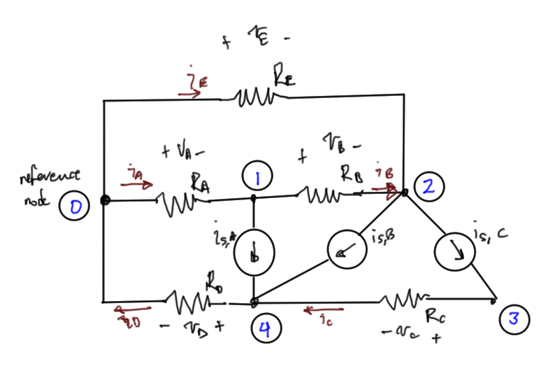
Avoiding branch currents can reduce the scope of the computational problem. Consider the same circuit fig. 1, this time introducing only node voltages as unknowns
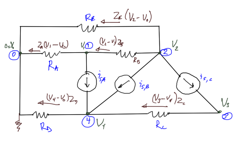
fig. 1. Resistive circuit with current sources
Unknowns: node voltages: \(V_1, V_2, \cdots V_4\)
Equations are KCL at each node except \(0\).
-
\(
\frac{V_1 – 0}{R_A} +
\frac{V_1 – V_2}{R_B} + i_{S,A} = 0
\) -
\(
\frac{V_2 – 0}{R_E} +
\frac{V_2 – V_1}{R_B} + i_{S,B} + i_{S,C} = 0
\) -
\(
\frac{V_3 – V_4}{R_C} – i_{S,C} = 0
\) -
\(
\frac{V_4 – 0}{R_D}
+\frac{V_4 – V_3}{R_C}
– i_{S,A} – i_{S,B} = 0
\)
In matrix form this is
\begin{equation}\label{eqn:multiphysicsL3:20}
\begin{bmatrix}
\inv{R_A} + \inv{R_B} & – \inv{R_B} & 0 & 0 \\
-\inv{R_B} & \inv{R_B} + \inv{R_E} & 0 & 0 \\
0 & 0 & \inv{R_C} & -\inv{R_C} \\
0 & 0 & -\inv{R_C} & \inv{R_C} + \inv{R_D}
\end{bmatrix}
\begin{bmatrix}
V_1 \\
V_2 \\
V_3 \\
V_4 \\
\end{bmatrix}
=
\begin{bmatrix}
-i_{S,A} \\
-i_{S,B} – i_{S,C} \\
i_{S,C} \\
i_{S,A} + i_{S,B}
\end{bmatrix}
\end{equation}
Introducing the nodal matrix
\begin{equation}\label{eqn:multiphysicsL3:40}
G \overline{{V}}_N = \overline{{I}}_S
\end{equation}
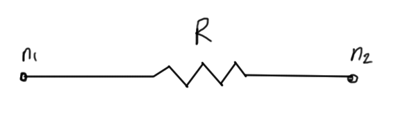
We identify the {stamp} for a resister of value \(R\) between nodes \(n_1\) and \(n_2\)
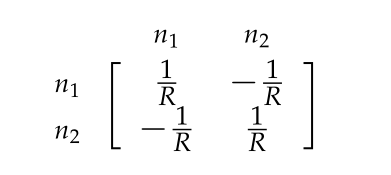
stamp matrix
where we have a set of rows and columns for each of the node voltages \(n_1, n_2\).
Note that some care is required to use this nodal analysis method since we required the invertible relationship \(i = V/R\). We also cannot handle short circuits \(V = 0\), or voltage sources \(V = 5\) (say). We will also have trouble with differential terms like inductors.
Recap of node branch equations
We had
- KCL: \( A \cdot \overline{{I}}_B = \overline{{I}}_S\)
- Constitutive: \( \overline{{I}}_B = \alpha A^\T \overline{{V}}_N \),
- Nodal equations: \( A \alpha A^\T \overline{{V}}_N = \overline{{I}}_S \)
where \(\overline{{I}}_B\) was the branch currents, \(A\) was the incidence matrix, and \(\alpha = \begin{bmatrix}\inv{R_1} & & \\ & \inv{R_2} & \\ & & \ddots \end{bmatrix} \).
The stamp can be observed in the multiplication of the contribution for a single resistor, where we see that the incidence matrix has the form \( G = A \alpha A^\T \)
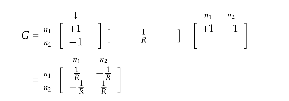
stamp factor
Theoretical facts
Noting that \(\lr{ A B }^\T = B^\T A^\T \), it is clear that the nodal matrix \(G = A \alpha A^\T \) is symmetric
\begin{equation}\label{eqn:multiphysicsL3:80}
G^\T
=
\lr{ A \alpha A^\T }^\T
=
\lr{ A^\T }^\T \alpha^\T A^\T
=
A \alpha A^\T
= G
\end{equation}
Modified nodal analysis (MNA)
This is the method that we find in software such as spice.
To illustrate the method, consider the same circuit, augmented with an additional voltage sources as in fig. 4.
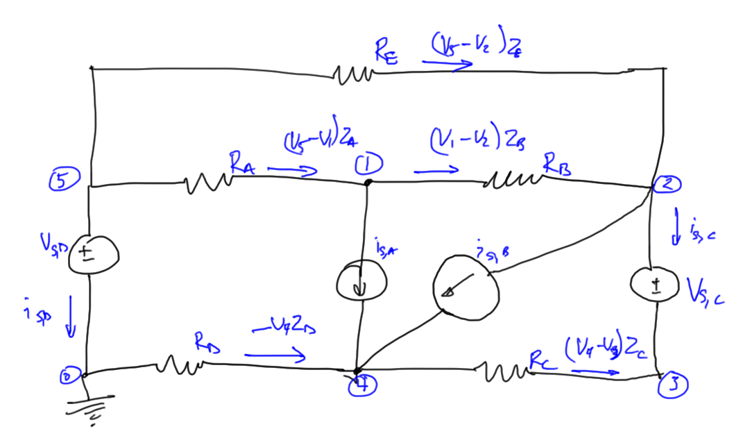
fig. 4. Resistive circuit with current and voltage sources
We know wish to have the following unknowns
- node voltages (\(N-1\)): \( V_1, V_2, \cdots V_5 \)
- branch currents for selected components (\(K\)): \( i_{S,C}, i_{S,D} \)
We will have two less unknowns for this system than with standard nodal analysis. Our equations are
-
\(
-\frac{V_5-V_1}{R_A}
+\frac{V_1-V_2}{R_B}
+ i_{S,A} = 0
\) -
\(
\frac{V_2-V_5}{R_E}
+\frac{V_2-V_1}{R_B}
+ i_{S,B}
+ i_{S,C}
= 0
\) -
\(
-i_{S,C} +
\frac{V_3-V_4}{R_C} = 0
\) -
\(
\frac{V_4-0}{R_D}
+\frac{V_4-V_3}{R_C}
– i_{S,A}
– i_{S,B}
= 0
\) -
\(
\frac{V_5-V_2}{R_E}
+\frac{V_5-V_1}{R_A}
+ i_{S,D} = 0
\)
Put into giant matrix form, this is
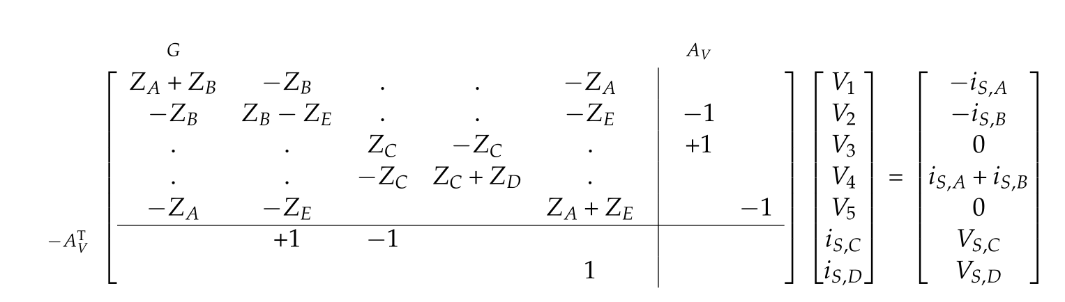
giant matrix
Call the extension to the nodal matrix \(G\), the {voltage incidence matrix} \(A_V\).