[Click here for a PDF of this post with nicer formatting]
Disclaimer
Peeter’s lecture notes from class. These may be incoherent and rough.
These are notes for the UofT course ECE1505H, Convex Optimization, taught by Prof. Stark Draper, from [1].
Topics
- Calculus: Derivatives and Jacobians, Gradients, Hessians, approximation functions.
- Linear algebra, Matrices, decompositions, …
Norms
Vector space:
A set of elements (vectors) that is closed under vector addition and scaling.
This generalizes the directed arrow concept of vector space (fig. 1) that is familiar from geometry.

fig. 1. Vector addition.
Normed vector spaces:
A vector space with a notion of length of any single vector, the “norm”.
Inner product space:
A normed vector space with a notion of a real angle between any pair of vectors.
This course has a focus on optimization in \R{n}. Complex spaces in the context of this course can be considered with a mapping \( \text{\C{n}} \rightarrow \mathbb{R}^{2 n} \).
Norm:
A norm is a function operating on a vector
\begin{equation*}
\Bx = ( x_1, x_2, \cdots, x_n )
\end{equation*}
that provides a mapping
\begin{equation*}
\Norm{ \cdot } : \mathbb{R}^{n} \rightarrow \mathbb{R},
\end{equation*}
where
- \( \Norm{ \Bx } \ge 0 \)
- \( \Norm{ \Bx } = 0 \qquad \iff \Bx = 0 \)
- \( \Norm{ t \Bx } = \Abs{t} \Norm{ \Bx } \)
- \( \Norm{ \Bx + \By } \le \Norm{ \Bx } + \Norm{\By} \). This is the triangle inequality.
Example: Euclidean norm
\begin{equation}\label{eqn:convex-optimizationLecture2:24}
\Norm{\Bx} = \sqrt{ \sum_{i = 1}^n x_i^2 }
\end{equation}
Example: \(l_p\)-norms
\begin{equation}\label{eqn:convex-optimizationLecture2:44}
\Norm{\Bx}_p = \lr{ \sum_{i = 1}^n \Abs{x_i}^p }^{1/p}.
\end{equation}
For \( p = 1 \), this is
\begin{equation}\label{eqn:convex-optimizationLecture2:64}
\Norm{\Bx}_1 = \sum_{i = 1}^n \Abs{x_i},
\end{equation}
For \( p = 2 \), this is the Euclidean norm \ref{eqn:convex-optimizationLecture2:24}.
For \( p = \infty \), this is
\begin{equation}\label{eqn:convex-optimizationLecture2:324}
\Norm{\Bx}_\infty = \max_{i = 1}^n \Abs{x_i}.
\end{equation}
Unit ball:
\begin{equation*}
\setlr{ \Bx | \Norm{\Bx} \le 1 }
\end{equation*}
The regions of the unit ball under the \( l_1, l_2, and l_\infty \) norms are plotted in fig. 2.
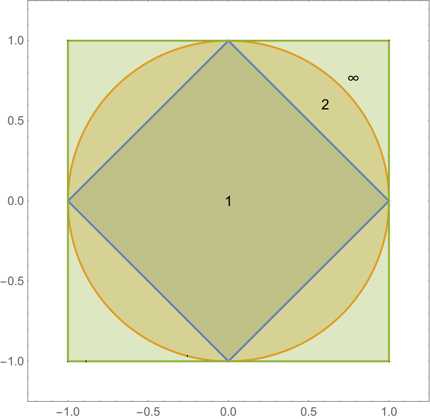
fig. 2. Some unit ball regions.
The \( l_2 \) norm is not only familiar, but can be “induced” by an inner product
\begin{equation}\label{eqn:convex-optimizationLecture2:84}
\left\langle \Bx, \By \right\rangle = \Bx^\T \By = \sum_{i = 1}^n x_i y_i,
\end{equation}
which is not true for all norms. The norm induced by this inner product is
\begin{equation}\label{eqn:convex-optimizationLecture2:104}
\Norm{\Bx}_2 = \sqrt{ \left\langle \Bx, \By \right\rangle }
\end{equation}
Inner product spaces have a notion of angle (fig. 3) given by
\begin{equation}\label{eqn:convex-optimizationLecture2:124}
\left\langle \Bx, \By \right\rangle = \Norm{\Bx} \Norm{\By} \cos \theta,
\end{equation}

fig. 3. Inner product induced angle.
and always satisfy the Cauchy-Schwartz inequality
\begin{equation}\label{eqn:convex-optimizationLecture2:144}
\left\langle \Bx, \By \right\rangle \le \Norm{\Bx}_2 \Norm{\By}_2.
\end{equation}
In an inner product space we say \( \Bx \) and \( \By \) are orthogonal vectors \( \Bx \perp \By \) if \( \left\langle \Bx, \By \right\rangle = 0 \), as sketched in fig. 4.

fig. 4. Orthogonality.
Dual norm
Let \( \Norm{ \cdot } \) be a norm in \R{n}. The “dual” norm \( \Norm{ \cdot }_\conj \) is defined as
\begin{equation*}
\Norm{\Bz}_\conj = \sup_\Bx \setlr{ \Bz^\T \Bx | \Norm{\Bx} \le 1 }.
\end{equation*}
where \( \sup \) is roughly the “least upper bound”.
\index{sup}
This is a limit over the unit ball of \( \Norm{\cdot} \).
\( l_2 \) dual
Dual of the \( l_2 \) is the \( l_2 \) norm.
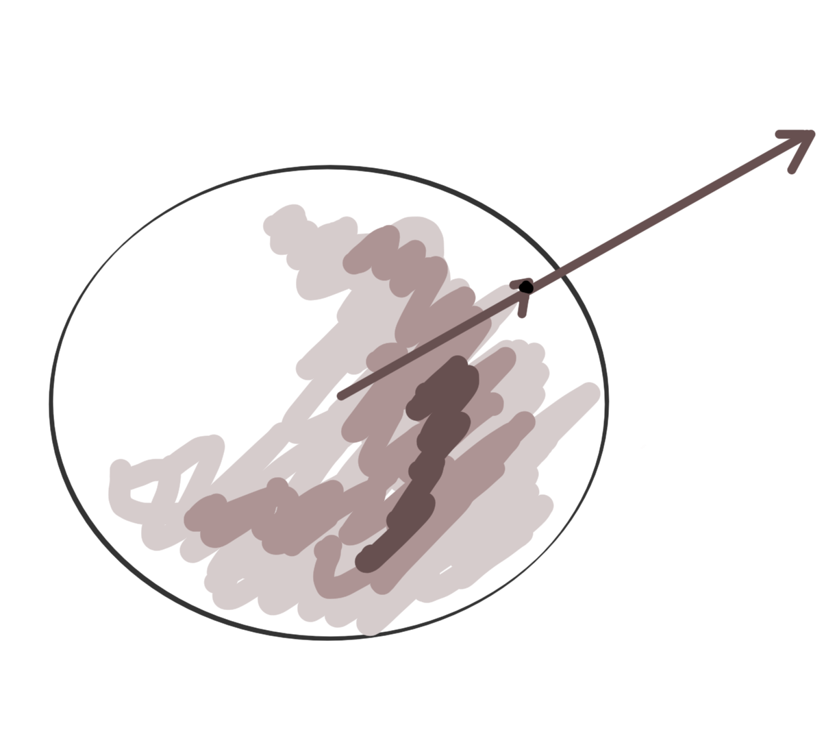
fig. 5. l_2 dual norm determination.
Proof:
\begin{equation}\label{eqn:convex-optimizationLecture2:164}
\begin{aligned}
\Norm{\Bz}_\conj
&= \sup_\Bx \setlr{ \Bz^\T \Bx | \Norm{\Bx}_2 \le 1 } \\
&= \sup_\Bx \setlr{ \Norm{\Bz}_2 \Norm{\Bx}_2 \cos\theta | \Norm{\Bx}_2 \le 1 } \\
&\le \sup_\Bx \setlr{ \Norm{\Bz}_2 \Norm{\Bx}_2 | \Norm{\Bx}_2 \le 1 } \\
&\le
\Norm{\Bz}_2
\Norm{
\frac{\Bz}{ \Norm{\Bz}_2 }
}_2 \\
&=
\Norm{\Bz}_2.
\end{aligned}
\end{equation}
\( l_1 \) dual
For \( l_1 \), the dual is the \( l_\infty \) norm. Proof:
\begin{equation}\label{eqn:convex-optimizationLecture2:184}
\Norm{\Bz}_\conj
=
\sup_\Bx \setlr{ \Bz^\T \Bx | \Norm{\Bx}_1 \le 1 },
\end{equation}
but
\begin{equation}\label{eqn:convex-optimizationLecture2:204}
\Bz^\T \Bx
=
\sum_{i=1}^n z_i x_i \le
\Abs{
\sum_{i=1}^n z_i x_i
}
\le
\sum_{i=1}^n \Abs{z_i x_i },
\end{equation}
so
\begin{equation}\label{eqn:convex-optimizationLecture2:224}
\begin{aligned}
\Norm{\Bz}_\conj
&=
\sum_{i=1}^n \Abs{z_i}\Abs{ x_i } \\
&\le \lr{ \max_{j=1}^n \Abs{z_j} }
\sum_{i=1}^n \Abs{ x_i } \\
&\le \lr{ \max_{j=1}^n \Abs{z_j} } \\
&=
\Norm{\Bz}_\infty.
\end{aligned}
\end{equation}
\( l_\infty \) dual
.

fig. 6. l_1 dual norm determination.
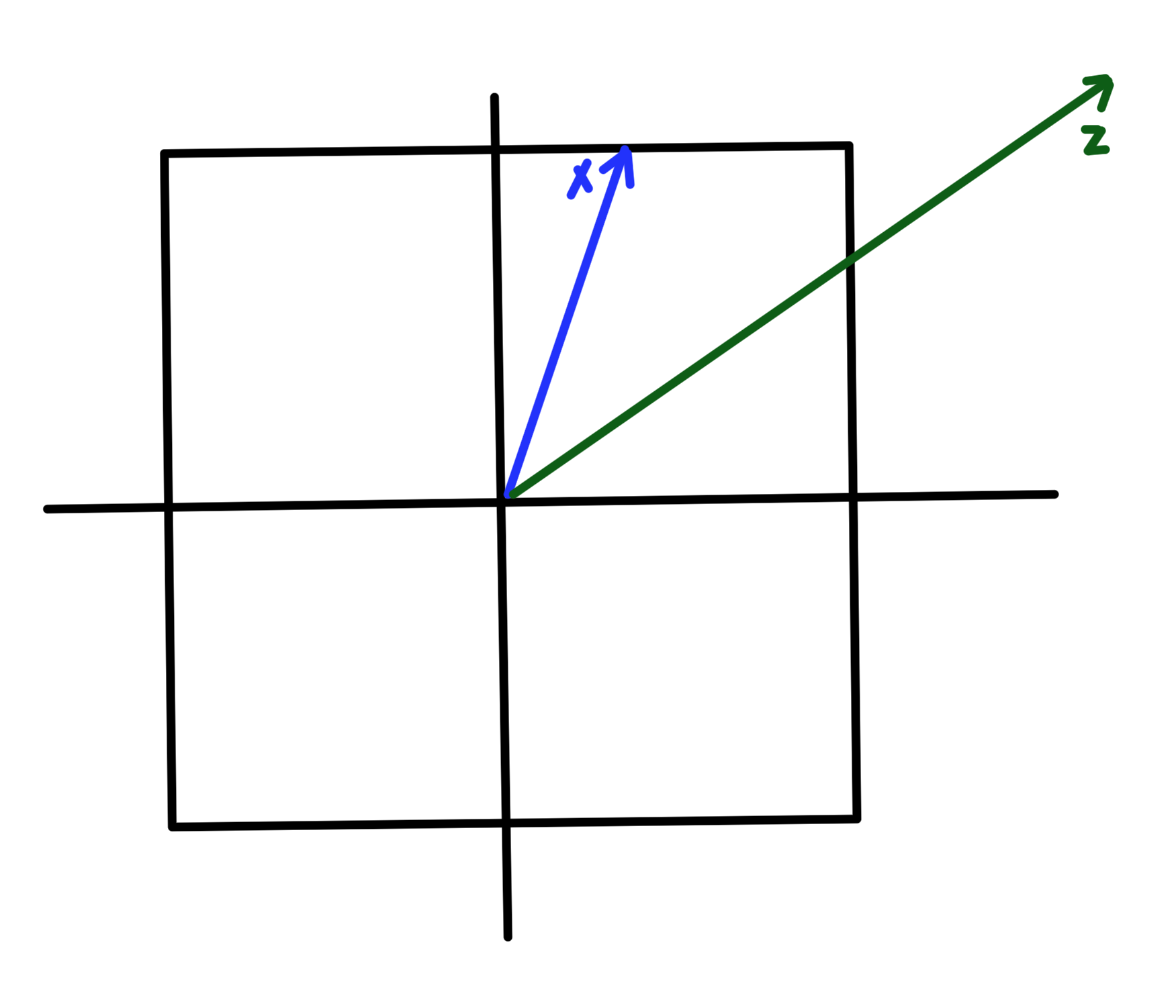
fig. 7. l_\infinity dual norm determination.
\begin{equation}\label{eqn:convex-optimizationLecture2:244}
\Norm{\Bz}_\conj
=
\sup_\Bx \setlr{ \Bz^\T \Bx | \Norm{\Bx}_\infty \le 1 }.
\end{equation}
Here
\begin{equation}\label{eqn:convex-optimizationLecture2:264}
\begin{aligned}
\Bz^\T \Bx
&=
\sum_{i=1}^n z_i x_i \\
&\le
\sum_{i=1}^n \Abs{z_i}\Abs{ x_i } \\
&\le
\lr{ \max_j \Abs{ x_j } }
\sum_{i=1}^n \Abs{z_i} \\
&=
\Norm{\Bx}_\infty
\sum_{i=1}^n \Abs{z_i}.
\end{aligned}
\end{equation}
So
\begin{equation}\label{eqn:convex-optimizationLecture2:284}
\Norm{\Bz}_\conj
\le
\sum_{i=1}^n \Abs{z_i}
=
\Norm{\Bz}_1.
\end{equation}
Statement from the lecture: I’m not sure where this fits:
\begin{equation}\label{eqn:convex-optimizationLecture2:304}
x_i^\conj
=
\left\{
\begin{array}{l l}
+1 & \quad \mbox{\( z_i \ge 0 \)} \\
-1 & \quad \mbox{\( z_i \le 0 \)}
\end{array}
\right.
\end{equation}
References
[1] Stephen Boyd and Lieven Vandenberghe. Convex optimization. Cambridge university press, 2004.