symmetry

PHY2403H Quantum Field Theory. Lecture 7: Symmetries, translation currents, energy momentum tensor. Taught by Prof. Erich Poppitz

October 3, 2018 phy2403 , , , , , ,

[Click here for a PDF of this post with nicer formatting]

DISCLAIMER: Very rough notes from class, with some additional side notes.

These are notes for the UofT course PHY2403H, Quantum Field Theory I, taught by Prof. Erich Poppitz fall 2018.

Symmetries

Given the complexities of the non-linear systems we want to investigate, examination of symmetries gives us simpler problems that we can solve.

  • “internal” symmetries. This means that the symmetries do not act on space time \( (\Bx, t) \). An example is
    \begin{equation}\label{eqn:qftLecture7:20}
    \phi^i =
    \begin{bmatrix}
    \psi_1 \\
    \psi_2 \\
    \vdots \\
    \psi_N \\
    \end{bmatrix}
    \end{equation}
    If we map \( \phi^i \rightarrow O^i_j \phi^j \) where \( O^\T O = 1 \), then we call this an internal symmetry.
    The corresponding Lagrangian density might be something like
    \begin{equation}\label{eqn:qftLecture7:40}
    \LL = \inv{2} \partial_\mu \Bphi \cdot \partial^\mu \Bphi – \frac{m^2}{2} \Bphi \cdot \Bphi – V(\Bphi \cdot \Bphi)
    \end{equation}

  • spacetime symmetries: Translations, rotations, boosts, dilatations. We will consider continuous symmetries, which can be defined as a succession of infinitesimal transformations.
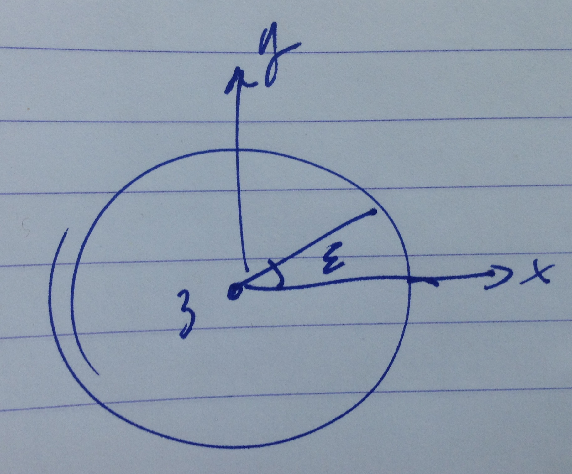
    An example from \(O(2)\) is a rotation
    \begin{equation}\label{eqn:qftLecture7:60}
    \begin{bmatrix}
    \phi^1 \\
    \phi^2 \\
    \end{bmatrix}
    \rightarrow
    \begin{bmatrix}
    \cos\alpha & \sin\alpha \\
    -\sin\alpha & \cos\alpha \\
    \end{bmatrix}
    \begin{bmatrix}
    \phi^1 \\
    \phi^2
    \end{bmatrix},
    \end{equation}
    or if \( \alpha \sim 0 \)
    \begin{equation}\label{eqn:qftLecture7:80}
    \begin{bmatrix}
    \phi^1 \\
    \phi^2 \\
    \end{bmatrix}
    \rightarrow
    \begin{bmatrix}
    1 & \alpha \\
    -\alpha & 1\\
    \end{bmatrix}
    \begin{bmatrix}
    \phi^1 \\
    \phi^2
    \end{bmatrix}
    =
    \begin{bmatrix}
    \phi^1 \\
    \phi^2
    \end{bmatrix}
    +
    \alpha
    \begin{bmatrix}
    \phi^2 \\
    -\phi^1
    \end{bmatrix}
    \end{equation}
    In index notation we write
    \begin{equation}\label{eqn:qftLecture7:100}
    \phi^i \rightarrow \phi^i + \alpha e^{ij} \phi^j,
    \end{equation}
    where \( \epsilon^{12} = +1, \epsilon^{21} = -1 \) is the completely antisymmetric tensor. This can be written in more general form as
    \begin{equation}\label{eqn:qftLecture7:120}
    \phi^i \rightarrow \phi^i + \delta \phi^i,
    \end{equation}
    where \( \delta \phi^i \) is considered to be an infinitesimal transformation.

Definition: Symmetry

A symmetry means that there is some transformation
\begin{equation*}
\phi^i \rightarrow \phi^i + \delta \phi^i,
\end{equation*}
where \( \delta \phi^i \) is an infinitesimal transformation, and the equations of motion are invariant under this transformation.

Theorem: Noether’s theorem (1st).

If the equations of motion re invariant under \( \phi^\mu \rightarrow \phi^\mu + \delta \phi^\mu \), then there exists a conserved current \( j^\mu \) such that \( \partial_\mu j^\mu = 0 \).

Noether’s first theorem applies to global symmetries, where the parameters are the same for all \( (\Bx, t)\). Gauge symmetries are not examples of such global symmetries.

Given a Lagrangian density \( \LL(\phi(x), \phi_{,\mu}(x)) \), where \( \phi_{,\mu} \equiv \partial_\mu \phi \). The action is
\begin{equation}\label{eqn:qftLecture7:160}
S = \int d^d x \LL.
\end{equation}
EOMs are invariant if under \( \phi(x) \rightarrow \phi'(x) = \phi(x) + \delta_\epsilon \phi(x)\), we have
\begin{equation}\label{eqn:qftLecture7:180}
\LL(\phi) \rightarrow \LL'(\phi’) = \LL(\phi) + \partial_\mu J_\epsilon^\mu(\phi) + O(\epsilon^2).
\end{equation}
Then there exists a conserved current. In QFT we say that the E.O.M’s are “on shell”. Note that \ref{eqn:qftLecture7:180} is a symmetry since we have added a total derivative to the Lagrangian which leaves the equations of motion of unchanged.

In general, the change of action under arbitrary variation of \( \delta \phi\) of the fields is
\begin{equation}\label{eqn:qftLecture7:200}
\begin{aligned}
\delta S
&=
\int d^d x \delta \LL(\phi, \partial_\mu \phi) \\
&=
\int d^d x \lr{
\PD{\phi}{\LL} \delta \phi
+
\PD{(\partial_\mu \phi)}{\LL} \delta \partial_\mu \phi
} \\
&=
\int d^d x \lr{
\partial_\mu \lr{ \PD{(\partial_\mu \phi)}{\LL} } \delta \phi
+
\PD{(\partial_\mu \phi)}{\LL} \partial_\mu \delta \phi
} \\
&=
\int d^d x
\partial_\mu \lr{ \frac{\delta \LL}{\delta(\partial_\mu \phi)} \delta \phi }
\end{aligned}
\end{equation}
However from \ref{eqn:qftLecture7:180}
\begin{equation}\label{eqn:qftLecture7:220}
\delta_\epsilon \LL = \partial_\mu J_\epsilon^\mu(\phi, \partial_\mu \phi),
\end{equation}
so after equating these variations we fine that
\begin{equation}\label{eqn:qftLecture7:240}
\delta S = \int d^d x \delta_\epsilon \LL = \int d^d x \partial_\mu J_\epsilon^\mu,
\end{equation}
or
\begin{equation}\label{eqn:qftLecture7:260}
0 = \int d^d x
\partial_\mu \lr{ \frac{\delta \LL}{\delta(\partial_\mu \phi)} \delta \phi – J_\epsilon^\mu },
\end{equation}
or \( \partial_\mu j^\mu = 0 \) provided
\begin{equation}\label{eqn:qftLecture7:280}
\boxed{
j^\mu =
\frac{\delta \LL}{\delta(\partial_\mu \phi)} \delta_\epsilon \phi – J_\epsilon^\mu.
}
\end{equation}

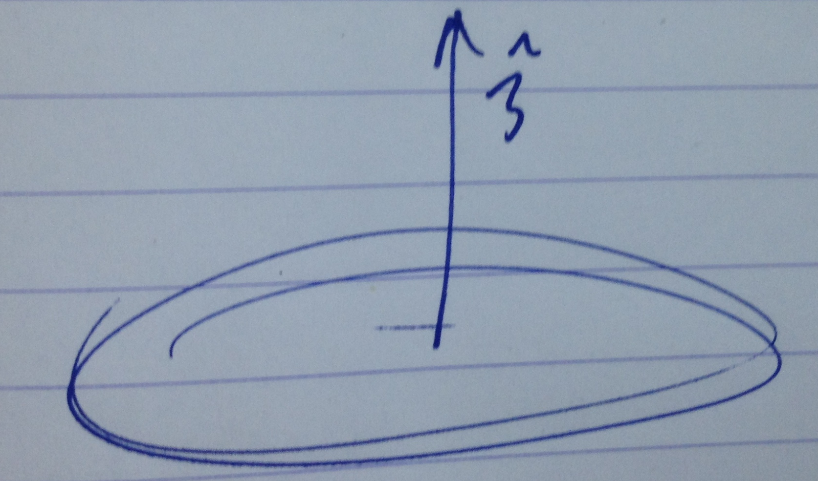
Integrating the divergence of the current over a space time volume, perhaps that of cylinder (time up, space out) is also zero. That is
\begin{equation}\label{eqn:qftLecture7:300}
\begin{aligned}
0
&=
\int d^4 x \, \partial_\mu j^\mu \\
&=
\int d^3 \Bx dt \, \partial_\mu j^\mu \\
&=
\int d^3 \Bx dt \, \partial_t j^0 –
\int d^3 \Bx dt \spacegrad \cdot \Bj \\
&=
\int d^3 \Bx dt \, \partial_t j^0 ,
\end{aligned}
\end{equation}
where the spatial divergence is zero assuming there’s no current leaving the volume on the infinite boundary
(no \(\Bj\) at spatial infinity.)

We write
\begin{equation}\label{eqn:qftLecture7:560}
Q = \int d^3x \partial_t j^0,
\end{equation}
and call this the on-shell charge associated with the symmetry.

Spacetime translation.

A spacetime translation has the form
\begin{equation}\label{eqn:qftLecture7:320}
x^\mu \rightarrow {x’}^\mu = x^\mu + a^\mu,
\end{equation}
\begin{equation}\label{eqn:qftLecture7:340}
\phi(x) \rightarrow \phi'(x’) = \phi(x)
\end{equation}
(contrast this to a Lorentz transformation that had the form \( x^\mu \rightarrow {x’}^\mu = {\Lambda^\mu}_\nu x^\nu \)).

If \(\phi'(x + a) = \phi(x) \), then
\begin{equation}\label{eqn:qftLecture7:360}
\phi'(x) + a^\mu \partial_\mu \phi'(x) =
\phi'(x) + a^\mu \partial_\mu \phi(x) =
\phi(x),
\end{equation}
so
\begin{equation}\label{eqn:qftLecture7:380}
\phi'(x)
= \phi(x) – a^\mu \partial_\mu \phi'(x)
= \phi(x) + \delta_a \phi(x),
\end{equation}
or
\begin{equation}\label{eqn:qftLecture7:580}
\delta_a \phi(x) = – a^\mu \partial_\mu \phi(x).
\end{equation}
Under \( \phi \rightarrow \phi – a^\mu \partial_\mu \phi \), we have
\begin{equation}\label{eqn:qftLecture7:400}
\LL(\phi) \rightarrow \LL(\phi) – a^\mu \partial_\mu \LL.
\end{equation}
Let’s calculate this with our scalar theory Lagrangian
\begin{equation}\label{eqn:qftLecture7:420}
\LL = \inv{2} \partial_\mu \phi \partial^\mu \phi – \frac{m^2}{2} \phi^2 – V(\phi)
\end{equation}
The Lagrangian variation is
\begin{equation}\label{eqn:qftLecture7:440}
\begin{aligned}
\evalbar{\delta \LL}{\phi \rightarrow \phi + \delta \phi, \delta\phi = – a^\mu \partial_\mu \phi}
&=
(\partial_\mu \phi) \delta (\partial^\mu \phi) – m^2 \phi \delta \phi – \PD{\phi}{V} \delta \phi \\
&=
(\partial_\mu \phi)(-a^\nu \partial_\nu \phi \partial^\mu \phi) + m^2 \phi a^\nu \partial_\nu \phi + \PD{\phi}{V} a^\nu \partial_\nu \phi \\
&=
– a^\nu \partial_\nu \lr{ \inv{2} \partial_\mu \partial^\mu \phi – \frac{m^2}{2} \phi^2 – V(\phi) } \\
&=
– a^\nu \partial_\nu \LL.
\end{aligned}
\end{equation}

So the current is
\begin{equation}\label{eqn:qftLecture7:600}
\begin{aligned}
j^\mu
&=
(\partial^\mu \phi) (-a^\nu \partial_\nu \phi) + a^\nu \LL \\
&=
-a^\nu \lr{ \partial^\mu \phi \partial_\nu \phi – \LL }
\end{aligned}
\end{equation}

We really have a current for each \( \nu \) direction and can make that explicit writing
\begin{equation}\label{eqn:qftLecture7:460}
\begin{aligned}
\delta_\nu \LL
&= -\partial_\nu \LL \\
&= – \partial_\mu \lr{ {\delta^\mu}_\nu \LL } \\
&= \partial_\mu {J^\mu}_\nu
\end{aligned}
\end{equation}
we write
\begin{equation}\label{eqn:qftLecture7:480}
{j^\mu}_\nu = \PD{x_\mu}{\phi} \lr{ – \PD{x^\nu}{\phi} } + {\delta^\mu}_\nu \LL,
\end{equation}
where \( \nu \) are labels which coordinates are translated:
\begin{equation}\label{eqn:qftLecture7:500}
\begin{aligned}
\partial_\nu \phi &= – \partial_\nu \phi \\
\partial_\nu \LL &= – \partial_\nu \LL.
\end{aligned}
\end{equation}
We call the conserved quantities elements of the energy-momentum tensor, and write it as
\begin{equation}\label{eqn:qftLecture7:520}
\boxed{
{T^\mu}_\nu = -\PD{x_\mu}{\phi} \PD{x^\nu}{\phi} + {\delta^\mu}_\nu \LL.
}
\end{equation}

Incidentally, we picked a non-standard sign convention for the tensor, as an explicit expansion of \( T^{00} \), the energy density component, shows
\begin{equation}\label{eqn:qftLecture7:540}
\begin{aligned}
{T^0}_0
&=
-\PD{t}{\phi}
\PD{t}{\phi}
+\inv{2}
\PD{t}{\phi}
\PD{t}{\phi}
– \inv{2} (\spacegrad \phi) \cdot (\spacegrad \phi)
– \frac{m^2}{2} \phi^2 – V(\phi) \\
&=
-\inv{2} \PD{t}{\phi} \PD{t}{\phi}
– \inv{2} (\spacegrad \phi) \cdot (\spacegrad \phi)
– \frac{m^2}{2} \phi^2 – V(\phi).
\end{aligned}
\end{equation}
Had we translated by \( -a^\mu \) we’d have a positive definite tensor instead.

Third update of aggregate notes for phy1520, Graduate Quantum Mechanics.

November 9, 2015 phy1520 , , , , , , , , , , , , , , , ,

I’ve posted a third update of my aggregate notes for PHY1520H Graduate Quantum Mechanics, taught by Prof. Arun Paramekanti. In addition to what was noted previously, this contains lecture notes up to lecture 13, my solutions for the third problem set, and some additional worked practice problems.

Most of the content was posted individually in the following locations, but those original documents will not be maintained individually any further.

PHY1520H Graduate Quantum Mechanics. Lecture 12: Symmetry (cont.). Taught by Prof. Arun Paramekanti

November 5, 2015 phy1520 , , , , , , ,

[Click here for a PDF of this post with nicer formatting]

Disclaimer

Peeter’s lecture notes from class. These may be incoherent and rough.

These are notes for the UofT course PHY1520, Graduate Quantum Mechanics, taught by Prof. Paramekanti, covering chap. 4 content from [1].

Parity (review)

\begin{equation}\label{eqn:qmLecture12:20}
\hat{\Pi} \hat{x} \hat{\Pi} = – \hat{x}
\end{equation}
\begin{equation}\label{eqn:qmLecture12:40}
\hat{\Pi} \hat{p} \hat{\Pi} = – \hat{p}
\end{equation}

These are polar vectors, in contrast to an axial vector such as \( \BL = \Br \cross \Bp \).

\begin{equation}\label{eqn:qmLecture12:60}
\hat{\Pi}^2 = 1
\end{equation}

\begin{equation}\label{eqn:qmLecture12:80}
\Psi(x) \rightarrow \Psi(-x)
\end{equation}

If \( \antisymmetric{\hat{\Pi}}{\hat{H}} = 0 \) then all the eigenstates are either

  • even: \( \hat{\Pi} \) eigenvalue is \( + 1 \).
  • odd: \( \hat{\Pi} \) eigenvalue is \( – 1 \).

We are done with discrete symmetry operators for now.

Translations

Define a (continuous) translation operator

\begin{equation}\label{eqn:qmLecture12:100}
\hat{T}_\epsilon \ket{x} = \ket{x + \epsilon}
\end{equation}

The action of this operator is sketched in fig. 1.

lecture12Fig1

fig. 1. Translation operation.


This is a unitary operator

\begin{equation}\label{eqn:qmLecture12:120}
\hat{T}_{-\epsilon} = \hat{T}_{\epsilon}^\dagger = \hat{T}_{\epsilon}^{-1}
\end{equation}

In a position basis, the action of this operator is

\begin{equation}\label{eqn:qmLecture12:140}
\bra{x} \hat{T}_{\epsilon} \ket{\psi} = \braket{x-\epsilon}{\psi} = \psi(x – \epsilon)
\end{equation}

\begin{equation}\label{eqn:qmLecture12:160}
\Psi(x – \epsilon) \approx \Psi(x) – \epsilon \PD{x}{\Psi}
\end{equation}

\begin{equation}\label{eqn:qmLecture12:180}
\bra{x} \hat{T}_{\epsilon} \ket{\Psi}
= \braket{x}{\Psi} – \frac{\epsilon}{\Hbar} \bra{ x} i \hat{p} \ket{\Psi}
\end{equation}

\begin{equation}\label{eqn:qmLecture12:200}
\hat{T}_{\epsilon} \approx \lr{ 1 – i \frac{\epsilon}{\Hbar} \hat{p} }
\end{equation}

A non-infinitesimal translation can be composed of many small translations, as sketched in fig. 2.

fig. 2. Composition of small translations

fig. 2. Composition of small translations

For \( \epsilon \rightarrow 0, N \rightarrow \infty, N \epsilon = a \), the total translation operator is

\begin{equation}\label{eqn:qmLecture12:220}
\begin{aligned}
\hat{T}_{a}
&= \hat{T}_{\epsilon}^N \\
&= \lim_{\epsilon \rightarrow 0, N \rightarrow \infty, N \epsilon = a }
\lr{ 1 – \frac{\epsilon}{\Hbar} \hat{p} }^N \\
&= e^{-i a \hat{p}/\Hbar}
\end{aligned}
\end{equation}

The momentum \( \hat{p} \) is called a “Generator” generator of translations. If a Hamiltonian \( H \) is translationally invariant, then

\begin{equation}\label{eqn:qmLecture12:240}
\antisymmetric{\hat{T}_{a}}{H} = 0, \qquad \forall a.
\end{equation}

This means that momentum will be a good quantum number

\begin{equation}\label{eqn:qmLecture12:260}
\antisymmetric{\hat{p}}{H} = 0.
\end{equation}

Rotations

Rotations form a non-Abelian group, since the order of rotations \( \hatR_1 \hatR_2 \ne \hatR_2 \hatR_1 \).

Given a rotation acting on a ket

\begin{equation}\label{eqn:qmLecture12:280}
\hatR \ket{\Br} = \ket{R \Br},
\end{equation}

observe that the action of the rotation operator on a wave function is inverted

\begin{equation}\label{eqn:qmLecture12:300}
\bra{\Br} \hatR \ket{\Psi}
=
\bra{R^{-1} \Br} \ket{\Psi}
= \Psi(R^{-1} \Br).
\end{equation}

Example: Z axis normal rotation

Consider an infinitesimal rotation about the z-axis as sketched in fig. 3(a),(b)

lecture12Fig3

fig 3(a). Rotation about z-axis.

fig 3(b). Rotation about z-axis.

fig 3(b). Rotation about z-axis.

\begin{equation}\label{eqn:qmLecture12:320}
\begin{aligned}
x’ &= x – \epsilon y \\
y’ &= y + \epsilon y \\
z’ &= z
\end{aligned}
\end{equation}

The rotated wave function is

\begin{equation}\label{eqn:qmLecture12:340}
\tilde{\Psi}(x,y,z)
= \Psi( x + \epsilon y, y – \epsilon x, z )
=
\Psi( x, y, z )
+
\epsilon y \underbrace{\PD{x}{\Psi}}_{i \hat{p}_x/\Hbar}

\epsilon x \underbrace{\PD{y}{\Psi}}_{i \hat{p}_y/\Hbar}.
\end{equation}

The state must then transform as

\begin{equation}\label{eqn:qmLecture12:360}
\ket{\tilde{\Psi}}
=
\lr{
1
+ i \frac{\epsilon}{\Hbar} \hat{y} \hat{p}_x
– i \frac{\epsilon}{\Hbar} \hat{x} \hat{p}_y
}
\ket{\Psi}.
\end{equation}

Observe that the combination \( \hat{x} \hat{p}_y – \hat{y} \hat{p}_x \) is the \( \hat{L}_z \) component of angular momentum \( \hat{\BL} = \hat{\Br} \cross \hat{\Bp} \), so the infinitesimal rotation can be written

\begin{equation}\label{eqn:qmLecture12:380}
\boxed{
\hatR_z(\epsilon) \ket{\Psi}
=
\lr{ 1 – i \frac{\epsilon}{\Hbar} \hat{L}_z } \ket{\Psi}.
}
\end{equation}

For a finite rotation \( \epsilon \rightarrow 0, N \rightarrow \infty, \phi = \epsilon N \), the total rotation is

\begin{equation}\label{eqn:qmLecture12:420}
\hatR_z(\phi)
=
\lr{ 1 – \frac{i \epsilon}{\Hbar} \hat{L}_z }^N,
\end{equation}

or
\begin{equation}\label{eqn:qmLecture12:440}
\boxed{
\hatR_z(\phi)
=
e^{-i \frac{\phi}{\Hbar} \hat{L}_z}.
}
\end{equation}

Note that \( \antisymmetric{\hat{L}_x}{\hat{L}_y} \ne 0 \).

By construction using Euler angles or any other method, a general rotation will include contributions from components of all the angular momentum operator, and will have the structure

\begin{equation}\label{eqn:qmLecture12:480}
\boxed{
\hatR_\ncap(\phi)
=
e^{-i \frac{\phi}{\Hbar} \lr{ \hat{\BL} \cdot \ncap }}.
}
\end{equation}

Rotationally invariant \( \hat{H} \).

Given a rotationally invariant Hamiltonian

\begin{equation}\label{eqn:qmLecture12:520}
\antisymmetric{\hat{R}_\ncap(\phi)}{\hat{H}} = 0 \qquad \forall \ncap, \phi,
\end{equation}

then every

\begin{equation}\label{eqn:qmLecture12:540}
\antisymmetric{\BL \cdot \ncap}{\hat{H}} = 0,
\end{equation}

or
\begin{equation}\label{eqn:qmLecture12:560}
\antisymmetric{L_i}{\hat{H}} = 0,
\end{equation}

Non-Abelian implies degeneracies in the spectrum.

Time-reversal

Imagine that we have something moving along a curve at time \( t = 0 \), and ending up at the final position at time \( t = t_f \).

fig. 4. Time reversal trajectory.

fig. 4. Time reversal trajectory.

Imagine that we flip the direction of motion (i.e. flipping the velocity) and run time backwards so the final-time state becomes the initial state.

If the time reversal operator is designated \( \hat{\Theta} \), with operation

\begin{equation}\label{eqn:qmLecture12:580}
\hat{\Theta} \ket{\Psi} = \ket{\tilde{\Psi}},
\end{equation}

so that

\begin{equation}\label{eqn:qmLecture12:600}
\hat{\Theta}^{-1} e^{-i \hat{H} t/\Hbar} \hat{\Theta} \ket{\Psi(t)} = \ket{\Psi(0)},
\end{equation}

or

\begin{equation}\label{eqn:qmLecture12:620}
\hat{\Theta}^{-1} e^{-i \hat{H} t/\Hbar} \hat{\Theta} \ket{\Psi(0)} = \ket{\Psi(-t)}.
\end{equation}

References

[1] Jun John Sakurai and Jim J Napolitano. Modern quantum mechanics. Pearson Higher Ed, 2014.

PHY1520H Graduate Quantum Mechanics. Lecture 11: Symmetries in QM. Taught by Prof. Arun Paramekanti

October 29, 2015 phy1520 , ,

[Click here for a PDF of this post with nicer formatting]

Disclaimer

Peeter’s lecture notes from class. These may be incoherent and rough.

These are notes for the UofT course PHY1520, Graduate Quantum Mechanics, taught by Prof. Paramekanti, covering \textchapref{{4}} [1] content.

Symmetry in classical mechanics

In a classical context considering a Hamiltonian

\begin{equation}\label{eqn:qmLecture11:20}
H(q_i, p_i),
\end{equation}

a symmetry means that certain \( q_i \) don’t appear. In that case the rate of change of one of the generalized momenta is zero

\begin{equation}\label{eqn:qmLecture11:40}
\ddt{p_k} = – \PD{q_k}{H} = 0,
\end{equation}

so \( p_k \) is a constant of motion. This simplifies the problem by reducing the number of degrees of freedom. Another aspect of such a symmetry is that it \underline{relates trajectories}. For example, assuming a rotational symmetry as in fig. 1.

fig. 1.  Trajectory under rotational symmetry

fig. 1. Trajectory under rotational symmetry

the trajectory of a particle after rotation is related by rotation to the trajectory of the unrotated particle.

Symmetry in quantum mechanics

Suppose that we have a symmetry operation that takes states from

\begin{equation}\label{eqn:qmLecture11:60}
\ket{\psi} \rightarrow \ket{U \psi}
\end{equation}
\begin{equation}\label{eqn:qmLecture11:80}
\ket{\phi} \rightarrow \ket{U \phi},
\end{equation}

we expect that

\begin{equation}\label{eqn:qmLecture11:100}
\Abs{\braket{ \psi}{\phi} }^2 = \Abs{\braket{ U\psi}{ U\phi} }^2.
\end{equation}

This won’t hold true for a general operator. Two cases where this does hold true is when

  • \( \braket{\psi}{\phi} = \braket{ U\psi}{ U\phi} \). Here \( U \) is unitary, and the equivalence follows from

    \begin{equation}\label{eqn:qmLecture11:120}
    \braket{ U\psi}{ U\phi} = \bra{ \psi} U^\dagger U { \phi} = \bra{ \psi} 1 { \phi} = \braket{\psi}{\phi}.
    \end{equation}

  • \( \braket{\psi}{\phi} = \braket{ U\psi}{ U\phi}^\conj \). Here \( U \) is anti-unitary.

Unitary case

If an “observable” is not changed by a unitary operation representing a symmetry we must have

\begin{equation}\label{eqn:qmLecture11:140}
\bra{\psi} \hat{A} \ket{\psi}
\rightarrow
\bra{U \psi} \hat{A} \ket{U \psi}
=
\bra{\psi} U^\dagger \hat{A} U \ket{\psi},
\end{equation}

so
\begin{equation}\label{eqn:qmLecture11:160}
U^\dagger \hat{A} U = \hat{A},
\end{equation}

or
\begin{equation}\label{eqn:qmLecture11:180}
\boxed{
\hat{A} U = U \hat{A}.
}
\end{equation}

An observable that is unchanged by a unitary symmetry commutes \( \antisymmetric{\hat{A}}{U} \) with the operator \( U \) for that transformation.

Symmetries of the Hamiltonian

Given
\begin{equation}\label{eqn:qmLecture11:200}
\antisymmetric{H}{U} = 0,
\end{equation}

\( H \) is invariant.

Given

\begin{equation}\label{eqn:qmLecture11:220}
H \ket{\phi_n} = \epsilon_n \ket{\phi_n} .
\end{equation}

\begin{equation}\label{eqn:qmLecture11:240}
\begin{aligned}
U H \ket{\phi_n}
&= H U \ket{\phi_n} \\
&= \epsilon_n U \ket{\phi_n}
\end{aligned}
\end{equation}

Such a state

\begin{equation}\label{eqn:qmLecture11:260}
\ket{\psi_n} = U \ket{\phi_n}
\end{equation}

is also an eigenstate with the \underline{same} energy.

Suppose this process is repeated, finding other states

\begin{equation}\label{eqn:qmLecture11:280}
U \ket{\psi_n} = \ket{\chi_n}
\end{equation}
\begin{equation}\label{eqn:qmLecture11:300}
U \ket{\chi_n} = \ket{\alpha_n}
\end{equation}

Because such a transformation only generates states with the initial energy, this process cannot continue forever. At some point this process will enumerate a fixed size set of states. These states can be orthonormalized.

We can say that symmetry operations are generators of a \underlineAndIndex{group}. For a set of symmetry operations we can

  • Form products that lie in a closed set

    \begin{equation}\label{eqn:qmLecture11:320}
    U_1 U_2 = U_3
    \end{equation}

  • can define an inverse
    \begin{equation}\label{eqn:qmLecture11:340}
    U \leftrightarrow U^{-1}.
    \end{equation}

  • obeys associative rules for multiplication
    \begin{equation}\label{eqn:qmLecture11:360}
    U_1 ( U_2 U_3 ) = (U_1 U_2) U_3.
    \end{equation}

  • has an identity operation.

When \( H \) has a symmetry, then degenerate eigenstates form \underlineAndIndex{irreducible} representations (which cannot be further block diagonalized).

Some simple examples

Example: Inversion.

{example:qmLecture11:1}

Given a state and a parity operation \( \hat{\Pi} \), with the transformation

\begin{equation}\label{eqn:qmLecture11:380}
\ket{\psi} \rightarrow \hat{\Pi} \ket{\psi}
\end{equation}

In one dimension, the parity operation is just inversion. In two dimensions, this is a set of flipping operations on two axes fig. 2.

fig. 2.  2D parity operation

fig. 2. 2D parity operation

The operational effects of this operator are

\begin{equation}\label{eqn:qmLecture11:400}
\begin{aligned}
\hat{x} &\rightarrow – \hat{x} \\
\hat{p} &\rightarrow – \hat{p}.
\end{aligned}
\end{equation}

Acting again with the parity operator produces the original value, so it is its own inverse, and \( \hat{\Pi}^\dagger = \hat{\Pi} = \hat{\Pi}^{-1} \). In an expectation value

\begin{equation}\label{eqn:qmLecture11:420}
\bra{ \hat{\Pi} \psi } \hat{x} \ket{ \hat{\Pi} \psi } = – \bra{\psi} \hat{x} \ket{\psi}.
\end{equation}

This means that

\begin{equation}\label{eqn:qmLecture11:440}
\hat{\Pi}^\dagger \hat{x} \hat{\Pi} = – \hat{x},
\end{equation}

or
\begin{equation}\label{eqn:qmLecture11:460}
\hat{x} \hat{\Pi} = – \hat{\Pi} \hat{x},
\end{equation}

\begin{equation}\label{eqn:qmLecture11:480}
\begin{aligned}
\hat{x} \hat{\Pi} \ket{x_0}
&= – \hat{\Pi} \hat{x} \ket{x_0} \\
&= – \hat{\Pi} x_0 \ket{x_0} \\
&= – x_0 \hat{\Pi} \ket{x_0}
\end{aligned}
\end{equation}

so

\begin{equation}\label{eqn:qmLecture11:500}
\hat{\Pi} \ket{x_0} = \ket{-x_0}.
\end{equation}

Acting on a wave function

\begin{equation}\label{eqn:qmLecture11:520}
\begin{aligned}
\bra{x} \hat{\Pi} \ket{\psi}
&=
\braket{-x}{\psi} \\
&= \psi(-x).
\end{aligned}
\end{equation}

What does this mean for eigenfunctions. Eigenfunctions are supposed to form irreducible representations of the group. The group has just two elements

\begin{equation}\label{eqn:qmLecture11:540}
\setlr{ 1, \hat{\Pi} },
\end{equation}

where \( \hat{\Pi}^2 = 1 \).

Suppose we have a Hamiltonian

\begin{equation}\label{eqn:qmLecture11:560}
H = \frac{\hat{p}^2}{2m} + V(\hat{x}),
\end{equation}

where \( V(\hat{x}) \) is even ( \( \antisymmetric{V(\hat{x})}{\hat{\Pi} } = 0 \) ). The squared momentum commutes with the parity operator

\begin{equation}\label{eqn:qmLecture11:580}
\begin{aligned}
\antisymmetric{\hat{p}^2}{\hat{\Pi}}
&=
\hat{p}^2 \hat{\Pi}
– \hat{\Pi} \hat{p}^2 \\
&=
\hat{p}^2 \hat{\Pi}
– (\hat{\Pi} \hat{p}) \hat{p} \\
&=
\hat{p}^2 \hat{\Pi}
-(- \hat{p} \hat{\Pi}) \hat{p} \\
&=
\hat{p}^2 \hat{\Pi}
+ \hat{p} (-\hat{p} \hat{\Pi}) \\
&=
0.
\end{aligned}
\end{equation}

Only two functions are possible in the symmetry set \( \setlr{ \Psi(x), \hat{\Pi} \Psi(x) } \), since

\begin{equation}\label{eqn:qmLecture11:600}
\begin{aligned}
\hat{\Pi}^2 \Psi(x)
&= \hat{\Pi} \Psi(-x) \\
&= \Psi(x).
\end{aligned}
\end{equation}

This symmetry severely restricts the possible solutions, making it so there can be only one dimensional forms of this problem with solutions that are either even or odd respectively

\begin{equation}\label{eqn:qmLecture11:620}
\begin{aligned}
\phi_e(x) &= \psi(x ) + \psi(-x) \\
\phi_o(x) &= \psi(x ) – \psi(-x).
\end{aligned}
\end{equation}

References

[1] Jun John Sakurai and Jim J Napolitano. Modern quantum mechanics. Pearson Higher Ed, 2014.