[Click here for a PDF of this post with nicer formatting]
In order to apply the Fresnel equations, the field components have to be resolved into components where either the electric field or the magnetic field is parallel to the plane of reflection. The geometry of this, with the wave vector direction \( \kcap \) and the electric and magnetic field phasors perpendicular to that direction is sketched in fig. 1.
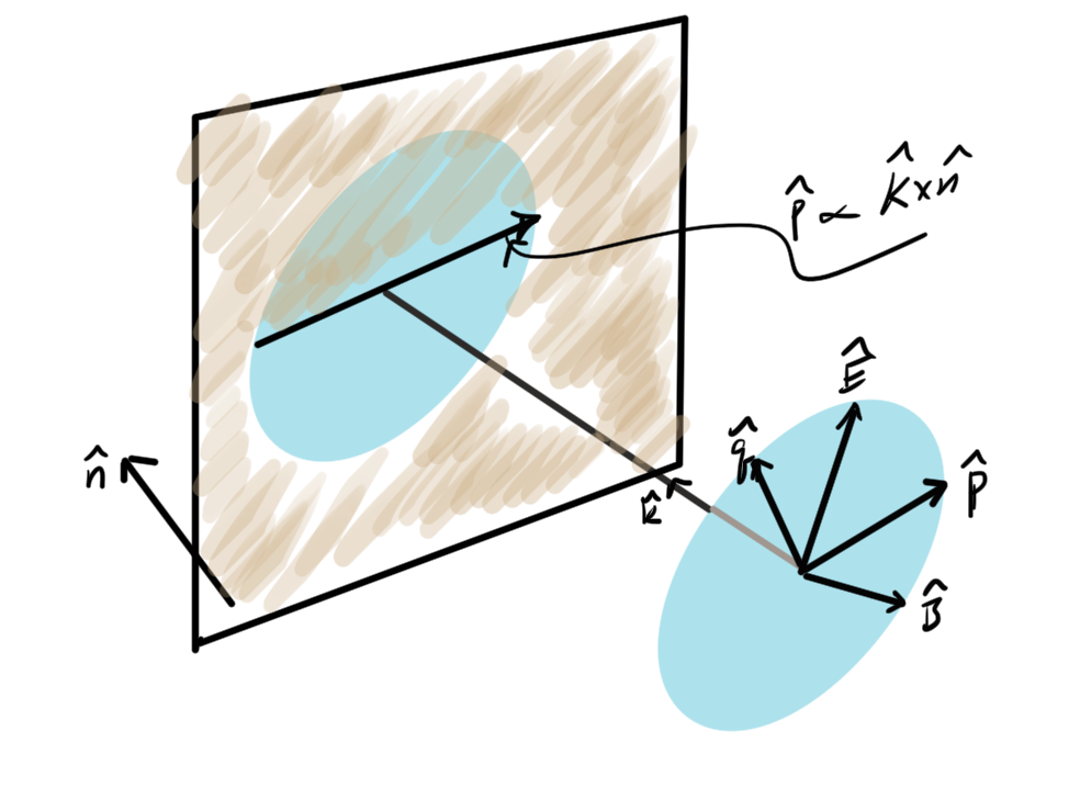
fig. 1. Field components relative to reflecting plane
If the incident wave is a plane wave, or equivalently a far field spherical wave, it will have the form
\begin{equation}\label{eqn:resolvingFieldsIncidentOnPlane:20}
\BH = \inv{\mu_0} \kcap \cross \BE,
\end{equation}
with the field directions and wave vector directions satisfying
\begin{equation}\label{eqn:resolvingFieldsIncidentOnPlane:60}
\Ecap \cross \Hcap = \kcap
\end{equation}
\begin{equation}\label{eqn:resolvingFieldsIncidentOnPlane:80}
\Ecap \cdot \kcap = 0
\end{equation}
\begin{equation}\label{eqn:resolvingFieldsIncidentOnPlane:100}
\Hcap \cdot \kcap = 0.
\end{equation}
The key to resolving the fields into components parallel to the plane of reflection lies in the observation that the cross product of the plane normal \( \ncap \) and the incident wave vector direction \( \kcap \) lies in that plane. With
\begin{equation}\label{eqn:resolvingFieldsIncidentOnPlane:140}
\pcap = \frac{\kcap \cross \ncap}{\Abs{\kcap \cross \ncap}}
\end{equation}
\begin{equation}\label{eqn:resolvingFieldsIncidentOnPlane:160}
\qcap = \kcap \cross \pcap,
\end{equation}
the field directions can be resolved into components
\begin{equation}\label{eqn:resolvingFieldsIncidentOnPlane:200}
\BE = \lr{ \BE \cdot \pcap } \pcap + \lr{ \BE \cdot \qcap } \qcap = E_\parallel \pcap + E_\perp \qcap
\end{equation}
\begin{equation}\label{eqn:resolvingFieldsIncidentOnPlane:220}
\BH = \lr{ \BH \cdot \pcap } \pcap + \lr{ \BH \cdot \qcap } \qcap = H_\parallel \pcap + H_\perp \qcap.
\end{equation}
This subdivides the fields into two pairs, one with the electric field parallel to the reflection plane
\begin{equation}\label{eqn:resolvingFieldsIncidentOnPlane:240}
\begin{aligned}
\BE_1 &= \lr{ \BE \cdot \pcap } \pcap = E_\parallel \pcap \\
\BH_1 &= \lr{ \BH \cdot \qcap } \qcap = H_\perp \qcap,
\end{aligned}
\end{equation}
and one with the magnetic field parallel to the reflection plane
\begin{equation}\label{eqn:resolvingFieldsIncidentOnPlane:260}
\begin{aligned}
\BH_2 &= \lr{ \BH \cdot \pcap } \pcap = H_\parallel \pcap \\
\BE_2 &= \lr{ \BE \cdot \qcap } \qcap = E_\perp \qcap.
\end{aligned}
\end{equation}
This is most of what we need to proceed with the reflection and transmission analysis. The only task remaining is to determine the reflection angle.
Using a pencil with the tip on the table I was able to convince myself by observation that there is always a normal plane of incidence regardless of any oblique angle that the ray hits the reflecting surface. This was, for some reason, not intuitively obvious to me. Having done that, the geometry must be reduced to what is sketched in fig. 2.
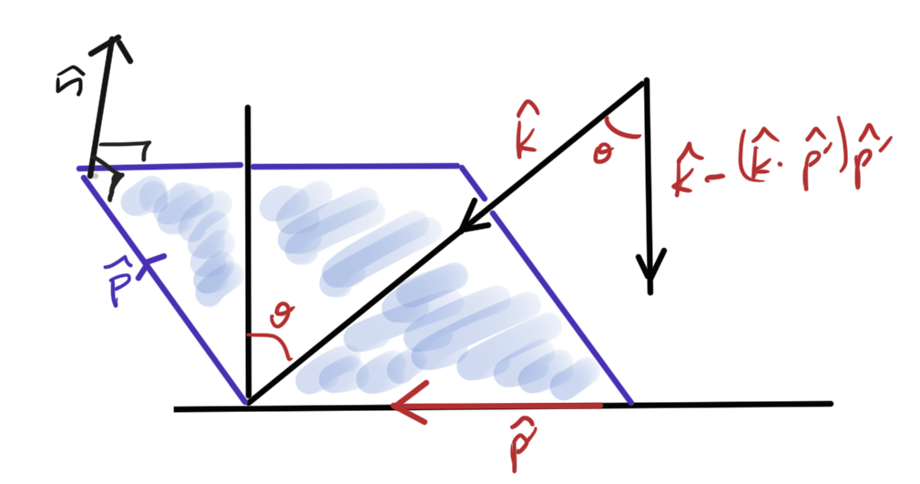
fig. 2. Angle of incidence determination
Once \( \pcap \) has been determined, regardless of it’s orientation in the reflection plane, the component of \( \kcap \) that is normal, directed towards, the plane of reflection is
\begin{equation}\label{eqn:resolvingFieldsIncidentOnPlane:280}
\kcap – \lr{ \kcap \cdot \pcap } \pcap,
\end{equation}
with (squared) length
\begin{equation}\label{eqn:resolvingFieldsIncidentOnPlane:300}
\begin{aligned}
\lr{ \kcap – \lr{ \kcap \cdot \pcap } \pcap }^2
&=
1 + \lr{ \kcap \cdot \pcap }^2 – 2 \lr{ \kcap \cdot \pcap }^2 \\
&=
1 – \lr{ \kcap \cdot \pcap }^2.
\end{aligned}
\end{equation}
The angle of incidence, relative to the normal to the reflection plane, follows from
\begin{equation}\label{eqn:resolvingFieldsIncidentOnPlane:320}
\begin{aligned}
\cos\theta
&= \kcap \cdot \frac{
\kcap – \lr{ \kcap \cdot \pcap } \pcap }{
\sqrt{
1 – \lr{ \kcap \cdot \pcap }^2
}
} \\
&=
\sqrt{
1 – \lr{ \kcap \cdot \pcap }^2
},
\end{aligned}
\end{equation}
Expanding the dot product above gives
\begin{equation}\label{eqn:resolvingFieldsIncidentOnPlane:360}
\begin{aligned}
\kcap \cdot \pcap’
&=
\kcap \cdot \lr{ \pcap \cross \ncap } \\
&=
\frac{1}{\Abs{\kcap \cross \ncap} } \kcap \cdot \lr{ \lr{\kcap \cross \ncap} \cross \ncap },
\end{aligned}
\end{equation}
where
\begin{equation}\label{eqn:resolvingFieldsIncidentOnPlane:380}
\begin{aligned}
\kcap \cdot \lr{ \lr{\kcap \cross \ncap} \cross \ncap }
&=
k_r \epsilon_{r s t} \lr{\kcap \cross \ncap}_s n_t \\
&=
k_r \epsilon_{r s t} \epsilon_{s a b} k_a n_b n_t \\
&=
-k_r \delta_{r t}^{[a b]} k_a n_b n_t \\
&=
-k_r n_t \lr{ k_r n_t – k_t n_r } \\
&=
-1 + \lr{ \kcap \cdot \ncap}^2.
\end{aligned}
\end{equation}
That gives
\begin{equation}\label{eqn:resolvingFieldsIncidentOnPlane:400}
\begin{aligned}
\kcap \cdot \pcap’
&=
\frac{-1 + \lr{ \kcap \cdot \ncap}^2}{\sqrt{1 – \lr{ \kcap \cdot \ncap}^2} } \\
&=
-\sqrt{1 – \lr{ \kcap \cdot \ncap}^2},
\end{aligned}
\end{equation}
or
\begin{equation}\label{eqn:resolvingFieldsIncidentOnPlane:420}
\begin{aligned}
\cos\theta
&= \sqrt{ 1 – \lr{-\sqrt{1 – \lr{ \kcap \cdot \ncap}^2}}^2 } \\
&= \sqrt{ \lr{ \kcap \cdot \ncap}^2 } \\
&= \kcap \cdot \ncap.
\end{aligned}
\end{equation}
This surprisingly simple result makes so much sense, it is an awful admission of stupidity that I went through all the vector algebra to get it instead of just writing it down directly.
The end result is the reflection angle is given by
\begin{equation}\label{eqn:resolvingFieldsIncidentOnPlane:340}
\boxed{
\theta = \cos^{-1} \kcap \cdot \ncap,
}
\end{equation}
where the reflection plane normal should off the back surface to get the sign right. The only detail left is the vector direction of the reflected ray (as well as the direction for the transmitted ray if that is of interest). The reflected ray direction flips the sign of the normal component of the ray
\begin{equation}\label{eqn:resolvingFieldsIncidentOnPlane:440}
\begin{aligned}
\kcap’
&= -\lr{\kcap \cdot \ncap} \ncap + \lr{ \kcap \wedge \ncap} \ncap \\
&= -\lr{\kcap \cdot \ncap} \ncap + \kcap – \lr{ \ncap \kcap} \cdot \ncap \\
&= \kcap -2 \lr{\kcap \cdot \ncap} \ncap.
\end{aligned}
\end{equation}
Here the sign of the normal doesn’t matter since it only occurs quadratically.
This now supplies everything needed for the application of the Fresnel equations to determine the reflected ray characteristics of an arbitrarily polarized incident field.