[Click here for a PDF version of this post]
I saw a thumbnail of a cube root simplification problem on youtube, and tried it myself before watching the video. I ended up needing two hints from the video to solve the problem. The problem was to simplify
\begin{equation}\label{eqn:cuberootsimplify:20}
x = \lr{ \sqrt{5} – 2 }^{1/3}.
\end{equation}
My guess was that the solution was of the form
\begin{equation}\label{eqn:cuberootsimplify:40}
x = a \sqrt{5} + b,
\end{equation}
where \(a,b\) are rational numbers. I say that because, if we cube that expression for \(x\) we get
\begin{equation}\label{eqn:cuberootsimplify:60}
x^3 = a^3 5 \sqrt{5} + 15 a^2 b + 3 \sqrt{5} a b^2 + b^3,
\end{equation}
so if we can find rational solutions to the system
\begin{equation}\label{eqn:cuberootsimplify:80}
\begin{aligned}
\sqrt{5} \lr{ 5 a^3 + 3 a b^2 } &= \sqrt{5} \\
15 a^2 b + b^3 &= -2.
\end{aligned}
\end{equation}
My problem now was that this doesn’t look like it’s particularly easy to solve. Mathematica can do it easily, as shown in fig. 1.
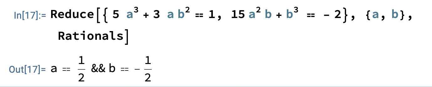
fig. 1. Mathematica simultaneous rational cubic reduction.
But if I wanted to cheat, I can just ask Mathematica to simplify the expression, as in fig. 2

fig. 2. Direct Mathematica simplification.
So, back to the drawing board. One thing that we can notice is that the expression in the cube root, looks like it could be recast in terms of a difference of squares
\begin{equation}\label{eqn:cuberootsimplify:100}
\sqrt{5} – 2 = \sqrt{5} – \sqrt{4}.
\end{equation}
Let’s let \( a = \sqrt{5}, b = \sqrt{4} \), so that
\begin{equation}\label{eqn:cuberootsimplify:120}
\begin{aligned}
\sqrt{5} – \sqrt{4} &=
a – b \\
&= \frac{a^2 – b^2}{a + b} \\
&= \frac{5 – 4}{\sqrt{5} + \sqrt{4} }.
\end{aligned}
\end{equation}
This shows that we have a sort of “conjugate” relationship for this difference
\begin{equation}\label{eqn:cuberootsimplify:140}
\sqrt{5} – 2 = \inv{\sqrt{5} + 2}.
\end{equation}
Surely this can be exploited somehow in the simplification process. I was stumped at this point, and didn’t see where to go with this, so I cheated a different way (not using Mathematica this time) and looked at the video to see where he went with it. Sure enough, he used these related pairs, and let
\begin{equation}\label{eqn:cuberootsimplify:160}
\begin{aligned}
x &= \lr{ \sqrt{5} – 2 }^{1/3} \\
y &= \lr{ \sqrt{5} + 2 }^{1/3}.
\end{aligned}
\end{equation}
Without looking further, let’s see what we can do with these. Clearly, we’d like to cube them, so that we seek solutions to
\begin{equation}\label{eqn:cuberootsimplify:180}
\begin{aligned}
x^3 &= \sqrt{5} – 2 \\
y^3 &= \sqrt{5} + 2.
\end{aligned}
\end{equation}
Sums and differences look like they would be interesting
\begin{equation}\label{eqn:cuberootsimplify:200}
\begin{aligned}
x^3 + y^3 &= 2 \sqrt{5} \\
y^3 – x^3 &= 4.
\end{aligned}
\end{equation}
We’ve also seen that
\begin{equation}\label{eqn:cuberootsimplify:220}
x y = 1,
\end{equation}
so just like the initial guess problem, we are left with having to solve two simulateous cubics, but this time the cubics are simpler, and we have a constraint condition that should be helpful.
My next guess was to form the cubes of \( x \pm y \), and use our constraint equation \( x y = 1 \) to simplify that. We find
\begin{equation}\label{eqn:cuberootsimplify:240}
\begin{aligned}
\lr{ x + y }^3
&= x^3 + 3 x^2 y + 3 x y^2 + y^3 \\
&= 2 \sqrt{5} + 3 \lr{ x + y} x y \\
&= 2 \sqrt{5} + 3 \lr{ x + y },
\end{aligned}
\end{equation}
and
\begin{equation}\label{eqn:cuberootsimplify:260}
\begin{aligned}
\lr{ y – x }^3
&= y^3 – 3 y^2 x + 3 y x^2 – x^3 \\
&= 4 – 3 \lr{ y – x } x y \\
&= 4 – 3 \lr{ y – x }.
\end{aligned}
\end{equation}
We can now let \( u = x + y, v = y – x \), and have a pair of independent equations to solve
\begin{equation}\label{eqn:cuberootsimplify:280}
\begin{aligned}
u^3 &= 2 \sqrt{5} + 3 u \\
v^3 &= 4 – 3 v.
\end{aligned}
\end{equation}
However, we still have cubic equations to solve, neither of which look particularly fun to reduce. I went around in circles from here and didn’t make much headway, and eventually went back to the video to see what he did. He ended up with an equivalent to my equation for \( v \) above, but I actually got there much more directly (my \( v \) was his \( -u \), so the exact steps he used differed.) His basic technique was to note that \( 4 = 3 + 1 \) so he looked for factors with \( 3 \) and \( 1 \) terms. In my case, that is equivalent to the observation that \( v = 1 \) is a root to the cubic in \( v \). So, we want to factor out \( v – 1 \) from
\begin{equation}\label{eqn:cuberootsimplify:300}
v^3 + 3 v – 4 = 0,
\end{equation}
Long dividing this by \( v -1 \) gives
\begin{equation}\label{eqn:cuberootsimplify:320}
\lr{ v – 1 } \lr{ v^2 + v + 4 } = 0.
\end{equation}
Completing the square for the quadratic factor gives
\begin{equation}\label{eqn:cuberootsimplify:340}
\lr{v + \inv{2} }^2 = -4 – \inv{4},
\end{equation}
which has only complex solutions (and we want a positive real solution.) Equating the remaining factor to zero, and reminding ourselves about our \( x y \) constraint, we are now left with
\begin{equation}\label{eqn:cuberootsimplify:360}
\begin{aligned}
v = y – x &= 1,
x y &= 1.
\end{aligned}
\end{equation}
Solving both for \( y \) gives
\begin{equation}\label{eqn:cuberootsimplify:380}
y = x + 1 = \inv{x},
\end{equation}
or
\begin{equation}\label{eqn:cuberootsimplify:400}
x^2 + x = 1,
\end{equation}
or
\begin{equation}\label{eqn:cuberootsimplify:420}
\lr{ x + \inv{2} }^2 = 1 – \inv{4} = \frac{5}{4}.
\end{equation}
We are left with two possible solutions for \( x \)
\begin{equation}\label{eqn:cuberootsimplify:440}
x = -\inv{2} \pm \frac{\sqrt{5}}{2},
\end{equation}
and we can now discard the negative solution, and find
\begin{equation}\label{eqn:cuberootsimplify:460}
x = \frac{ \sqrt{5} – 1 }{2},
\end{equation}
matching the answer that we’d found with the Mathematica cheat earlier.
Seeing the effort required to simplify this makes me impressed once again with Mathematica. I wonder what algorithm it uses to do the simplification?