angular momentum

New video: Elliptical motion from Newton’s law of gravitation.

September 14, 2023 math and physics play , , , , , , , , , ,

This blog post is a text version of the video below, available in a few forms:


We found previously that
\begin{equation}\label{eqn:solarellipse:20}
\mathbf{\hat{r}}’ = \inv{r} \mathbf{\hat{r}} \lr{ \mathbf{\hat{r}} \wedge \Bx’ }.
\end{equation}
Somewhat remarkably, we can use this identity to demonstrate that orbits governed gravitational force are elliptical (or parabolic, or hyperbolic.) This ends up being possible because the angular momentum of the system is a conserved quantity, and this immediately introduces angular momentum into the mix in a fundamental way. In particular,
\begin{equation}\label{eqn:solarellipse:40}
\mathbf{\hat{r}}’ = \inv{m r^2} \mathbf{\hat{r}} L,
\end{equation}
where we define the angular momentum bivector as
\begin{equation}\label{eqn:solarellipse:60}
L = \Bx \wedge \Bp.
\end{equation}
Our gravitational law is
\begin{equation}\label{eqn:solarellipse:80}
m \ddt{\Bv} = – G m M \frac{\mathbf{\hat{r}}}{r^2},
\end{equation}
or
\begin{equation}\label{eqn:solarellipse:100}
-\inv{G M} \ddt{\Bv} = \frac{\mathbf{\hat{r}}}{r^2}.
\end{equation}
Combining the gravitational law with our \( \mathbf{\hat{r}} \) derivative identity, we have
\begin{equation}\label{eqn:solarellipse:120}
\begin{aligned}
\ddt{ \mathbf{\hat{r}} }
&= \inv{m} \frac{\mathbf{\hat{r}}}{r^2} L \\
&= -\inv{G m M} \ddt{\Bv} L \\
&= -\inv{G m M} \lr{ \ddt{(\Bv L)} – \ddt{L} }.
\end{aligned}
\end{equation}
Since angular momentum is a constant of motion of the system, means that
\begin{equation}\label{eqn:solarellipse:140}
\ddt{L} = 0,
\end{equation}
our equation of motion is integratable
\begin{equation}\label{eqn:solarellipse:160}
\ddt{ \mathbf{\hat{r}} } = -\inv{G m M} \ddt{(\Bv L)}.
\end{equation}
Introducing a vector valued integration constant \( -\Be \), we have
\begin{equation}\label{eqn:solarellipse:180}
\mathbf{\hat{r}} = -\inv{G m M} \Bv L – \Be.
\end{equation}
We’ve transformed our second order differential equation to a first order equation, one that does not look easy to integrate one more time. Luckily, we do not have to integrate, and can partially solve this algebraically, enough to describe the orbit in a compact fashion.

Before trying that, it’s worth quickly demonstrating that this equation is not a multivector equation, but a vector equation, since the multivector \( \Bv L \) is, in fact, vector valued.
\begin{equation}\label{eqn:solarellipse:200}
\begin{aligned}
\Bv L
&= \Bv \lr{ \Bx \wedge (m \Bv) } \\
&\propto \mathbf{\hat{v}} \lr{ \mathbf{\hat{r}} \wedge \mathbf{\hat{v}} } \\
&= \mathbf{\hat{v}} \cdot \lr{ \mathbf{\hat{r}} \wedge \mathbf{\hat{v}} } + \mathbf{\hat{v}} \wedge \lr{ \mathbf{\hat{r}} \wedge \mathbf{\hat{v}} } \\
&= \mathbf{\hat{v}} \cdot \lr{ \mathbf{\hat{r}} \wedge \mathbf{\hat{v}} } \\
&= \lr{ \mathbf{\hat{v}} \cdot \mathbf{\hat{r}} } \mathbf{\hat{v}} – \mathbf{\hat{r}},
\end{aligned}
\end{equation}
which is a vector (i.e.: a vector that is directed along the portion of \( \Bx \) that is perpendicular to \( \Bv \).)

We can reduce \ref{eqn:solarellipse:180} to a scalar equation by dotting with \( \Bx = r \mathbf{\hat{r}} \), leaving
\begin{equation}\label{eqn:solarellipse:220}
\begin{aligned}
r
&= -\inv{G m M} \gpgradezero{ \Bx \Bv L } – \Bx \cdot \Be \\
&= -\inv{G m^2 M} \gpgradezero{ \Bx \Bp L } – \Bx \cdot \Be \\
&= -\inv{G m^2 M} \gpgradezero{ \lr{ \Bx \cdot \Bp + L } L } – \Bx \cdot \Be \\
&= -\inv{G m^2 M} L^2 – \Bx \cdot \Be,
\end{aligned}
\end{equation}
or
\begin{equation}\label{eqn:solarellipse:240}
r = -\frac{L^2}{G M m^2} – r e \cos\theta,
\end{equation}
or
\begin{equation}\label{eqn:solarellipse:260}
r \lr{ 1 + e \cos\theta } = -\frac{L^2}{G M m^2}.
\end{equation}
Observe that the RHS constant is a positive constant, since \( L^2 \le 0 \). This has the structure of a conic section, if we write
\begin{equation}\label{eqn:solarellipse:280}
-\frac{L^2}{G M m^2} = e d.
\end{equation}
This is an ellipse, for \( e \in [0,1) \), a parabola for \( e = 1 \), and hyperbola for \( e > 1 \) ([1] theorem 10.3.1).

fig. 1. Ellipse with e = 0.75

In fig. 1 is a plot with \( e = 0.75 \) (changing \( d \) doesn’t change the shape of the figure, just the size.)

References

[1] S.L. Salas and E. Hille. Calculus: one and several variables. Wiley New York, 1990.

Radial vector representation, momentum, and angular momentum.

September 8, 2023 math and physics play , , , , , ,

[Click here for a PDF version of this post], and here for a video version of this post.


Motivation.

In my last couple GA YouTube videos, circular and spherical coordinates were examined.

This post is a text representation of a new video that follows up on those two videos.

We found the form of the unit vector derivatives in both cases.

\begin{equation}\label{eqn:radialderivatives:20}
\Bx = r \mathbf{\hat{r}},
\end{equation}
leaving the angular dependence of \( \mathbf{\hat{r}} \) unspecified. We want to find both \( \Bv = \Bx’ \) and \( \mathbf{\hat{r}}’\).

Derivatives.

Lemma 1.1: Radial length derivative.

The derivative of a spherical length \( r \) can be expressed as
\begin{equation*}
\frac{dr}{dt} = \mathbf{\hat{r}} \cdot \frac{d\Bx}{dt}.
\end{equation*}

Start proof:

We write \( r^2 = \Bx \cdot \Bx \), and take derivatives of both sides, to find
\begin{equation}\label{eqn:radialderivatives:60}
2 r \frac{dr}{dt} = 2 \Bx \cdot \frac{d\Bx}{dt},
\end{equation}
or
\begin{equation}\label{eqn:radialderivatives:80}
\frac{dr}{dt} = \frac{\Bx}{r} \cdot \frac{d\Bx}{dt} = \mathbf{\hat{r}} \cdot \frac{d\Bx}{dt}.
\end{equation}

End proof.

Application of the chain rule to \ref{eqn:radialderivatives:20} is straightforward
\begin{equation}\label{eqn:radialderivatives:100}
\Bx’ = r’ \mathbf{\hat{r}} + r \mathbf{\hat{r}}’,
\end{equation}
but we don’t know the form for \( \mathbf{\hat{r}}’ \). We could proceed with a niave expansion of
\begin{equation}\label{eqn:radialderivatives:120}
\frac{d}{dt} \lr{ \frac{\Bx}{r} },
\end{equation}
but we can be sneaky, and perform a projective and rejective split of \( \Bx’ \) with respect to \( \mathbf{\hat{r}} \). That is
\begin{equation}\label{eqn:radialderivatives:140}
\begin{aligned}
\Bx’
&= \mathbf{\hat{r}} \mathbf{\hat{r}} \Bx’ \\
&= \mathbf{\hat{r}} \lr{ \mathbf{\hat{r}} \Bx’ } \\
&= \mathbf{\hat{r}} \lr{ \mathbf{\hat{r}} \cdot \Bx’ + \mathbf{\hat{r}} \wedge \Bx’} \\
&= \mathbf{\hat{r}} \lr{ r’ + \mathbf{\hat{r}} \wedge \Bx’}.
\end{aligned}
\end{equation}
We used our lemma in the last step above, and after distribution, find
\begin{equation}\label{eqn:radialderivatives:160}
\Bx’ = r’ \mathbf{\hat{r}} + \mathbf{\hat{r}} \lr{ \mathbf{\hat{r}} \wedge \Bx’ }.
\end{equation}
Comparing to \ref{eqn:radialderivatives:100}, we see that
\begin{equation}\label{eqn:radialderivatives:180}
r \mathbf{\hat{r}}’ = \mathbf{\hat{r}} \lr{ \mathbf{\hat{r}} \wedge \Bx’ }.
\end{equation}
We see that the radial unit vector derivative is proportional to the rejection of \( \mathbf{\hat{r}} \) from \( \Bx’ \)
\begin{equation}\label{eqn:radialderivatives:200}
\mathbf{\hat{r}}’ = \inv{r} \mathrm{Rej}_{\mathbf{\hat{r}}}(\Bx’) = \inv{r^3} \Bx \lr{ \Bx \wedge \Bx’ }.
\end{equation}
The vector \( \mathbf{\hat{r}}’ \) is perpendicular to \( \mathbf{\hat{r}} \) for any parameterization of it’s orientation, or in symbols
\begin{equation}\label{eqn:radialderivatives:220}
\mathbf{\hat{r}} \cdot \mathbf{\hat{r}}’ = 0.
\end{equation}
We saw this for the circular and spherical parameterizations, and see now that this also holds more generally.

Angular momentum.

Let’s now write out the momentum \( \Bp = m \Bv \) for a point particle with mass \( m \), and determine the kinetic energy \( m \Bv^2/2 = \Bp^2/2m \) for that particle.

The momentum is
\begin{equation}\label{eqn:radialderivatives:320}
\begin{aligned}
\Bp
&= m r’ \mathbf{\hat{r}} + m \mathbf{\hat{r}} \lr{ \mathbf{\hat{r}} \wedge \Bv } \\
&= m r’ \mathbf{\hat{r}} + \inv{r} \mathbf{\hat{r}} \lr{ \Br \wedge \Bp }.
\end{aligned}
\end{equation}
Observe that \( p_r = m r’ \) is the radial component of the momentum. It is natural to introduce a bivector valued angular momentum operator
\begin{equation}\label{eqn:radialderivatives:340}
L = \Br \wedge \Bp,
\end{equation}
splitting the momentum into a component that is strictly radial and a component that lies purely on the surface of a spherical surface in momentum space. That is
\begin{equation}\label{eqn:radialderivatives:360}
\Bp = p_r \mathbf{\hat{r}} + \inv{r} \mathbf{\hat{r}} L.
\end{equation}
Making use of the fact that \( \mathbf{\hat{r}} \) and \( \mathrm{Rej}_{\mathbf{\hat{r}}}(\Bx’) \) are perpendicular (so there are no cross terms when we square the momentum), the
kinetic energy is
\begin{equation}\label{eqn:radialderivatives:380}
\begin{aligned}
\inv{2m} \Bp^2
&= \inv{2m} \lr{ p_r \mathbf{\hat{r}} + \inv{r} \mathbf{\hat{r}} L }^2 \\
&= \inv{2m} p_r^2 + \inv{2 m r^2 } \mathbf{\hat{r}} L \mathbf{\hat{r}} L \\
&= \inv{2m} p_r^2 – \inv{2 m r^2 } \mathbf{\hat{r}} L^2 \mathbf{\hat{r}} \\
&= \inv{2m} p_r^2 – \inv{2 m r^2 } L^2 \mathbf{\hat{r}}^2,
\end{aligned}
\end{equation}
where we’ve used the anticommutative nature of \( \mathbf{\hat{r}} \) and \( L \) (i.e.: a sign swap is needed to swap them), and used the fact that \( L^2 \) is a scalar, allowing us to commute \( \mathbf{\hat{r}} \) with \( L^2 \). This leaves us with
\begin{equation}\label{eqn:radialderivatives:400}
E = \inv{2m} \Bp^2 = \inv{2m} p_r^2 – \inv{2 m r^2 } L^2.
\end{equation}
Observe that both the radial momentum term and the angular momentum term are both strictly postive, since \( L \) is a bivector and \( L^2 \le 0 \).

Problems.

Problem:

Find \ref{eqn:radialderivatives:200} without being sneaky.

Answer

\begin{equation}\label{eqn:radialderivatives:280}
\begin{aligned}
\mathbf{\hat{r}}’
&= \frac{d}{dt} \lr{ \frac{\Bx}{r} } \\
&= \inv{r} \Bx’ – \inv{r^2} \Bx r’ \\
&= \inv{r} \Bx’ – \inv{r} \mathbf{\hat{r}} r’ \\
&= \inv{r} \lr{ \Bx’ – \mathbf{\hat{r}} r’ } \\
&= \inv{r} \lr{ \mathbf{\hat{r}} \mathbf{\hat{r}} \Bx’ – \mathbf{\hat{r}} r’ } \\
&= \inv{r} \mathbf{\hat{r}} \lr{ \mathbf{\hat{r}} \Bx’ – r’ } \\
&= \inv{r} \mathbf{\hat{r}} \lr{ \mathbf{\hat{r}} \Bx’ – \mathbf{\hat{r}} \cdot \Bx’ } \\
&= \inv{r} \mathbf{\hat{r}} \lr{ \mathbf{\hat{r}} \wedge \Bx’ }.
\end{aligned}
\end{equation}

Problem:

Show that \ref{eqn:radialderivatives:200} can be expressed as a triple vector cross product
\begin{equation}\label{eqn:radialderivatives:230}
\mathbf{\hat{r}}’ = \inv{r^3} \lr{ \Bx \cross \Bx’ } \cross \Bx,
\end{equation}

Answer

While this may be familiar from elementary calculus, such as in [1], we can show follows easily from our GA result
\begin{equation}\label{eqn:radialderivatives:300}
\begin{aligned}
\mathbf{\hat{r}}’
&= \inv{r} \mathbf{\hat{r}} \lr{ \mathbf{\hat{r}} \wedge \Bx’ } \\
&= \inv{r} \gpgradeone{ \mathbf{\hat{r}} \lr{ \mathbf{\hat{r}} \wedge \Bx’ } } \\
&= \inv{r} \gpgradeone{ \mathbf{\hat{r}} I \lr{ \mathbf{\hat{r}} \cross \Bx’ } } \\
&= \inv{r} \gpgradeone{ I \lr{ \mathbf{\hat{r}} \cdot \lr{ \mathbf{\hat{r}} \cross \Bx’ } + \mathbf{\hat{r}} \wedge \lr{ \mathbf{\hat{r}} \cross \Bx’ } } } \\
&= \inv{r} \gpgradeone{ I^2 \mathbf{\hat{r}} \cross \lr{ \mathbf{\hat{r}} \cross \Bx’ } } \\
&= \inv{r} \lr{ \mathbf{\hat{r}} \cross \Bx’ } \cross \mathbf{\hat{r}}.
\end{aligned}
\end{equation}

References

[1] S.L. Salas and E. Hille. Calculus: one and several variables. Wiley New York, 1990.

New video: Velocity and angular momentum with geometric algebra

September 7, 2023 math and physics play , , , , ,


In this video, we compute velocity in a radial representation \( \mathbf{x} = r \mathbf{\hat{r}} \).

We use a scalar radial coordinate \( r \), and leave all the angular dependence implicitly encoded in a radial unit vector \( \mathbf{\hat{r}} \).

We find the geometric algebra structure of the \( \mathbf{\hat{r}}’ \) in two different ways, to find

\( \mathbf{\hat{r}}’ = \frac{\mathbf{\hat{r}}}{r} \left( \mathbf{\hat{r}} \wedge \mathbf{\hat{x}}’ \right), \)

then derive the conventional triple vector cross product equivalent for reference:

\( \mathbf{\hat{r}}’ = \left( \mathbf{\hat{r}} \times \mathbf{\hat{x}}’ \right) \times \frac{\mathbf{\hat{r}}}{r}. \)

We then compute kinetic energy in this representation, and show how a bivector-valued angular momentum \( L = \mathbf{x} \wedge \mathbf{p} \), falls naturally from that computation, where we have

\( \frac{m}{2} \mathbf{v}^2 = \frac{1}{2 m} {(m r’)}^2 – \frac{1}{2 m r^2 } L^2. \)

Prerequisites: calculus (derivatives and chain rule), and geometric algebra basics (vector multiplication, commutation relationships for vectors and bivectors in a plane, wedge and cross product equivalencies, …)

Errata: at around 4:12 I used \( \mathbf{r} \) instead of \( \mathbf{x} \), then kept doing so every time after that when the value for \( L \) was stated.

As well as being posted to Google’s censorship-tube, this video can also be found on odysee.

Angular momentum bivector in cylindrical and spherical bases.

September 15, 2022 math and physics play , , , , , , ,

[Click here for a PDF version of this post]

Motivation

In a discord thread on the bivector group (a geometric algebra group chat), MoneyKills posts about trouble he has calculating the correct expression for the angular momentum bivector or it’s dual.

This blog post is a more long winded answer than my bivector response and includes this calculation using both cylindrical and spherical coordinates.

Cylindrical coordinates.

The position vector for any point on a plane can be expressed as
\begin{equation}\label{eqn:amomentum:20}
\Br = r \rcap,
\end{equation}
where \( \rcap = \rcap(\phi) \) encodes all the angular dependence of the position vector, and \( r \) is the length along that direction to our point, as illustrated in fig. 1.

fig. 1. Cylindrical coordinates position vector.

The radial unit vector has a compact GA representation
\begin{equation}\label{eqn:amomentum:40}
\rcap = \Be_1 e^{i\phi},
\end{equation}
where \( i = \Be_1 \Be_2 \).

The velocity (or momentum) will have both \( \rcap \) and \( \phicap \) dependence. By chain rule, that velocity is
\begin{equation}\label{eqn:amomentum:60}
\Bv = \dot{r} \rcap + r \dot{\rcap},
\end{equation}
where
\begin{equation}\label{eqn:amomentum:80}
\begin{aligned}
\dot{\rcap}
&= \Be_1 i e^{i\phi} \dot{\phi} \\
&= \Be_2 e^{i\phi} \dot{\phi} \\
&= \phicap \dot{\phi}.
\end{aligned}
\end{equation}
It is left to the reader to show that the vector designated \( \phicap \), is a unit vector and perpendicular to \( \rcap \) (Hint: compute the grade-0 selection of the product of the two to show that they are perpendicular.)

We can now compute the momentum, which is
\begin{equation}\label{eqn:amomentum:100}
\Bp = m \Bv = m \lr{ \dot{r} \rcap + r \dot{\phi} \phicap },
\end{equation}
and the angular momentum bivector
\begin{equation}\label{eqn:amomentum:120}
\begin{aligned}
L
&= \Br \wedge \Bp \\
&= m \lr{ r \rcap } \wedge \lr{ \dot{r} \rcap + r \dot{\phi} \phicap } \\
&= m r^2 \dot{\phi} \rcap \phicap.
\end{aligned}
\end{equation}

This has the \( m r^2 \dot{\phi} \) magnitude that the OP was seeking.

Spherical coordinates.

In spherical coordinates, our position vector is
\begin{equation}\label{eqn:amomentum:140}
\Br = r \lr{ \Be_1 \sin\theta \cos\phi + \Be_2 \sin\theta \sin\phi + \Be_3 \cos\theta },
\end{equation}
as sketched in fig. 2.

fig. 2. Spherical coordinates.

We can factor this into a more compact representation
\begin{equation}\label{eqn:amomentum:160}
\begin{aligned}
\Br
&= r \lr{ \sin\theta \Be_1 (\cos\phi + \Be_{12} \sin\phi ) + \Be_3 \cos\theta } \\
&= r \lr{ \sin\theta \Be_1 e^{\Be_{12} \phi } + \Be_3 \cos\theta } \\
&= r \Be_3 \lr{ \cos\theta + \sin\theta \Be_3 \Be_1 e^{\Be_{12} \phi } }.
\end{aligned}
\end{equation}

It is useful to name two of the bivector terms above, first, we write \( i \) for the azimuthal plane bivector sketched in fig. 3.

Spherical coordinates, azimuthal plane.

\begin{equation}\label{eqn:amomentum:180}
i = \Be_{12},
\end{equation}
and introduce a bivector \( j \) that encodes the \( \Be_3, \rcap \) plane as sketched in fig. 4.

Spherical coordinates, “j-plane”.

\begin{equation}\label{eqn:amomentum:200}
j = \Be_{31} e^{i \phi}.
\end{equation}

Having done so, we now have a compact representation for our position vector
\begin{equation}\label{eqn:amomentum:220}
\begin{aligned}
\Br
&= r \Be_3 \lr{ \cos\theta + j \sin\theta } \\
&= r \Be_3 e^{j \theta}.
\end{aligned}
\end{equation}

This provides us with a nice compact representation of the radial unit vector
\begin{equation}\label{eqn:amomentum:240}
\rcap = \Be_3 e^{j \theta}.
\end{equation}

Just as was the case in cylindrical coordinates, our azimuthal plane unit vector is
\begin{equation}\label{eqn:amomentum:280}
\phicap = \Be_2 e^{i\phi}.
\end{equation}

Now we want to compute the velocity vector. As was the case in cylindrical coordinates, we have
\begin{equation}\label{eqn:amomentum:300}
\Bv = \dot{r} \rcap + r \dot{\rcap},
\end{equation}
but now we need the spherical representation for the \( \rcap \) derivative, which is
\begin{equation}\label{eqn:amomentum:320}
\begin{aligned}
\dot{\rcap}
&=
\PD{\theta}{\rcap} \dot{\theta} + \PD{\phi}{\rcap} \dot{\phi} \\
&=
\Be_3 e^{j\theta} j \dot{\theta} + \Be_3 \sin\theta \PD{\phi}{j} \dot{\phi} \\
&=
\rcap j \dot{\theta} + \Be_3 \sin\theta j i \dot{\phi}.
\end{aligned}
\end{equation}
We can reduce the second multivector term without too much work
\begin{equation}\label{eqn:amomentum:340}
\begin{aligned}
\Be_3 j i
&=
\Be_3 \Be_{31} e^{i\phi} i \\
&=
\Be_3 \Be_{31} i e^{i\phi} \\
&=
\Be_{33112} e^{i\phi} \\
&=
\Be_{2} e^{i\phi} \\
&= \phicap,
\end{aligned}
\end{equation}
so we have
\begin{equation}\label{eqn:amomentum:360}
\dot{\rcap}
=
\rcap j \dot{\theta} + \sin\theta \phicap \dot{\phi}.
\end{equation}

The velocity is
\begin{equation}\label{eqn:amomentum:380}
\Bv = \dot{r} \rcap + r \lr{ \rcap j \dot{\theta} + \sin\theta \phicap \dot{\phi} }.
\end{equation}

Now we can finally compute the angular momentum bivector, which is
\begin{equation}\label{eqn:amomentum:400}
\begin{aligned}
L &=
\Br \wedge \Bp \\
&=
m r \rcap \wedge \lr{ \dot{r} \rcap + r \lr{ \rcap j \dot{\theta} + \sin\theta \phicap \dot{\phi} } } \\
&=
m r^2 \rcap \wedge \lr{ \rcap j \dot{\theta} + \sin\theta \phicap \dot{\phi} } \\
&=
m r^2 \gpgradetwo{ \rcap \lr{ \rcap j \dot{\theta} + \sin\theta \phicap \dot{\phi} } },
\end{aligned}
\end{equation}
which is just
\begin{equation}\label{eqn:amomentum:420}
L =
m r^2 \lr{ j \dot{\theta} + \sin\theta \rcap \phicap \dot{\phi} }.
\end{equation}

I was slightly surprised by this result, as I naively expected the cylindrical coordinate result. We have a \( m r^2 \rcap \phicap \dot{\phi} \) term, as was the case in cylindrical coordinates, but scaled down with a \( \sin\theta \) factor. However, this result does make sense. Consider for example, some fixed circular motion with \( \theta = \mathrm{constant} \), as sketched in fig. 5.

fig. 5. Circular motion for constant theta

The radius of this circle is actually \( r \sin\theta \), so the total angular momentum for that motion is scaled down to \( m r^2 \sin\theta \dot{\phi} \), smaller than the maximum circular angular momentum of \( m r^2 \dot{\phi} \) which occurs in the \( \theta = \pi/2 \) azimuthal plane. Similarly, if we have circular motion in the “j-plane”, sketched in fig. 6.

fig. 6. Circular motion for constant phi.

where \( \phi = \mathrm{constant} \), then our angular momentum is \( L = m r^2 j \dot{\theta} \).

PHY2403H Quantum Field Theory. Lecture 9: Unbroken and spontaneously broken symmetries, Higgs Lagrangian, scale invariance, Lorentz invariance, angular momentum quantization. Taught by Prof. Erich Poppitz

October 11, 2018 phy2403 , , , , , , , , , , , , , , ,

[Click here for a PDF of this post with nicer formatting (and a Mathematica listing that I didn’t include in this blog post’s latex export)]

DISCLAIMER: Very rough notes from class, with some additional side notes.

These are notes for the UofT course PHY2403H, Quantum Field Theory I, taught by Prof. Erich Poppitz fall 2018.

Last time

We followed a sequence of operations

  1. Noether’s theorem
  2. \( \rightarrow \) conserved currents
  3. \( \rightarrow \) charges (classical)
  4. \( \rightarrow \) “correspondence principle”
  5. \( \rightarrow \hatQ \)
  • Hermitian operators
  • “generators of symmetry”
    \begin{equation}\label{eqn:qftLecture9:20}
    \hatU(\alpha) = e^{i \alpha \hatQ}
    \end{equation}
    We found
    \begin{equation}\label{eqn:qftLecture9:40}
    \hatU(\alpha) \phihat \hatU^\dagger(\alpha) = \phihat + i \alpha \antisymmetric{\hatQ}{\phihat} + \cdots
    \end{equation}

Example: internal symmetries:

(non-spacetime), such as \( O(N)\) or \( U(1) \).

In QFT internal symmetries can have different “\underline{modes of realization}”.

    [I]

  1. “Wigner mode”. These are also called “unbroken symmetries”.
    \begin{equation}\label{eqn:qftLecture9:60}
    \hatQ \ket{0} = 0
    \end{equation}
    i.e. \( \hatU(\alpha) \ket{0} = 0 \).
    Ground state invariant. Formally \( :\hatQ: \) annihilates \( \ket{0} \).
    \( \antisymmetric{\hatQ}{\hatH} = 0 \) implies that all eigenstates are eigenstates of \( \hatQ \) in \( U(1) \). Example from HW 1
    \begin{equation}\label{eqn:qftLecture9:80}
    \hatQ = \text{“charge” under \( U(1) \)}.
    \end{equation}
    All states have definite charge, just live in QU.
  2. “Nambu-Goldstone mode” (Landau-ginsburg). This is also called a “spontaneously broken symmetry”\footnote{
    First encounter example (HWII, \( SU(2) \times SU(2) \rightarrow SU(2) \)). Here a \( U(1) \) spontaneous broken symmetry.}.
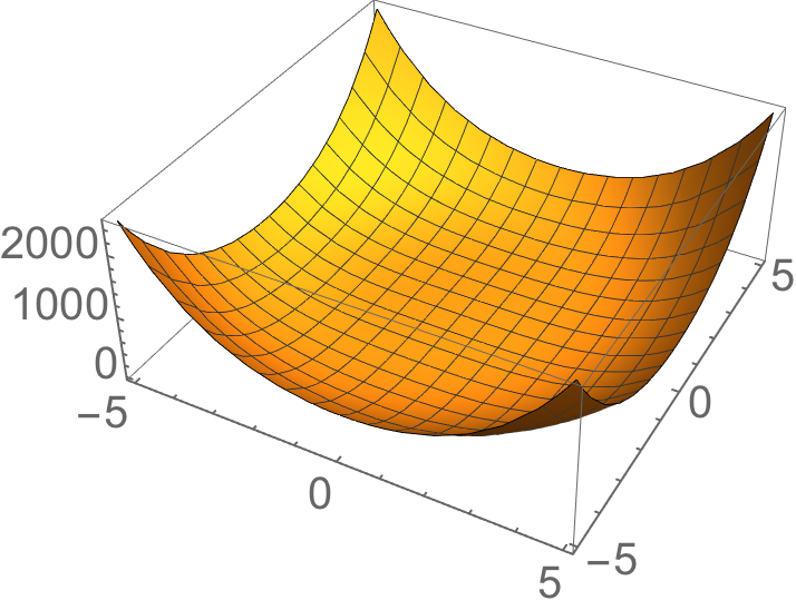
    \( H \) or \( L \) is invariant under symmetry, but ground state is not.

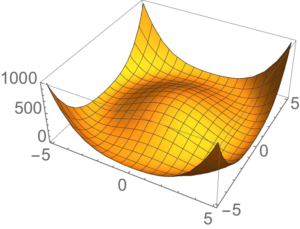
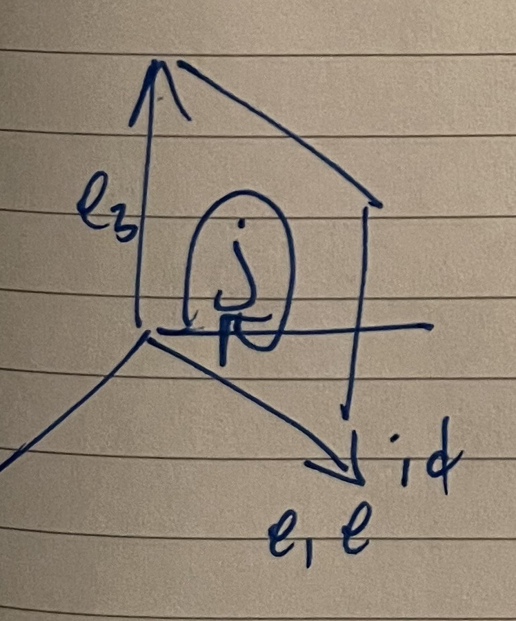
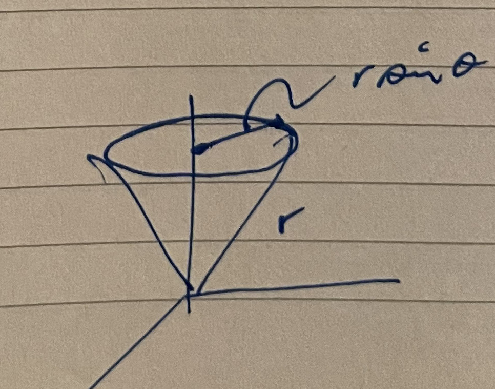
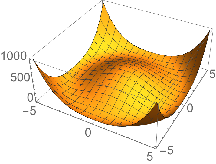
fig. 1. Mexican hat potential.

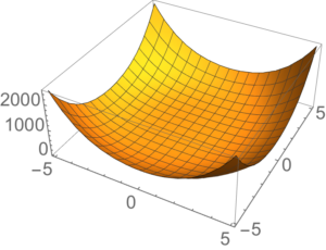
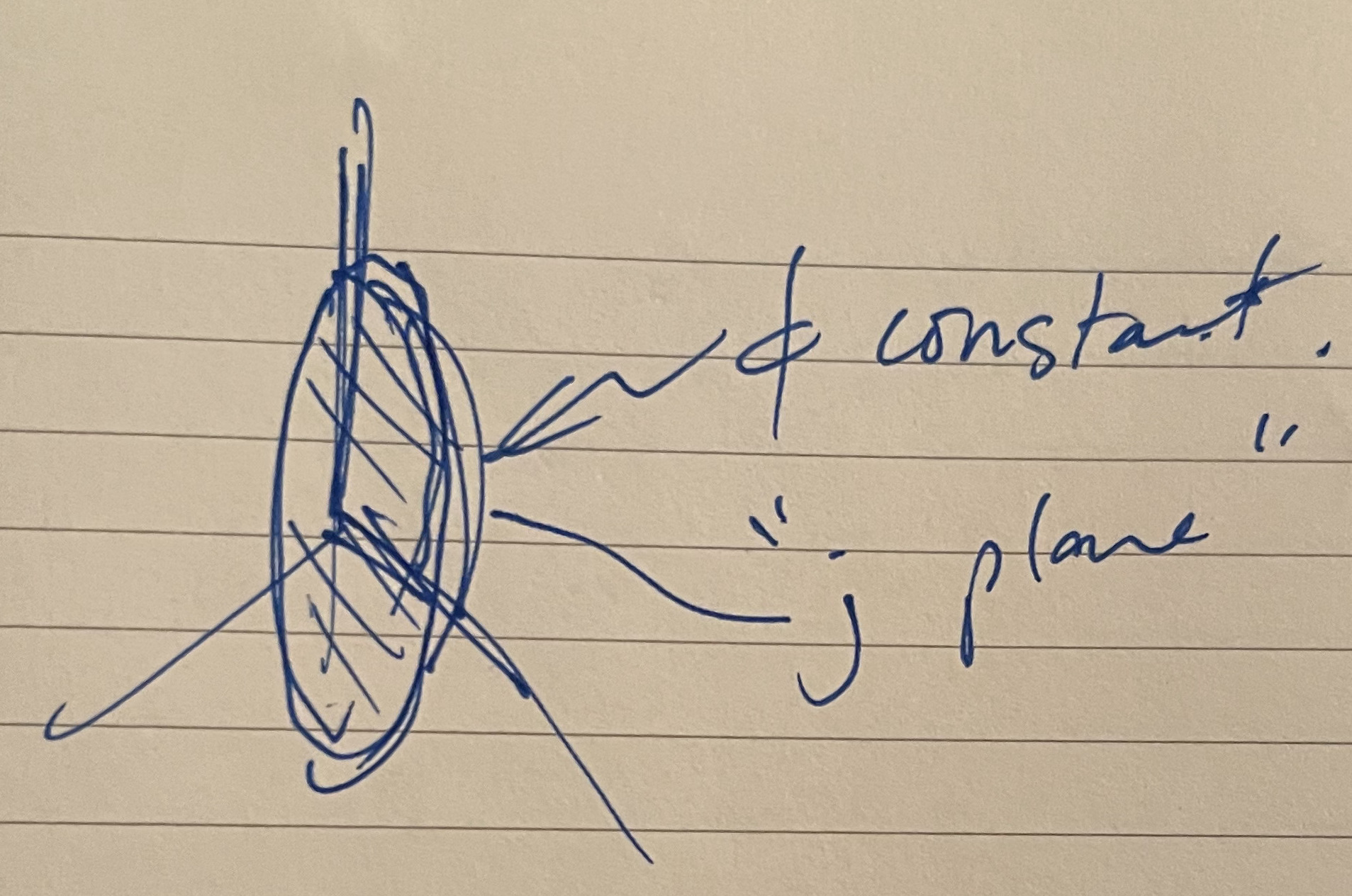
fig. 2. Degenerate Mexican hat potential ( v = 0)

Example:
\begin{equation}\label{eqn:qftLecture9:100}
\LL = \partial_\mu \phi^\conj \partial^\mu \phi – V(\Abs{\phi}),
\end{equation}
where
\begin{equation}\label{eqn:qftLecture9:120}
V(\Abs{\phi}) = m^2 \phi^\conj \phi + \frac{\lambda}{4} \lr{ \phi^\conj \phi }^2.
\end{equation}
When \( m^2 > 0 \) we have a Wigner mode, but when \( m^2 < 0 \) we have an issue: \( \phi = 0 \) is not a minimum of potential.
When \( m^2 < 0 \) we write
\begin{equation}\label{eqn:qftLecture9:140}
\begin{aligned}
V(\phi)
&= – m^2 \phi^\conj \phi + \frac{\lambda}{4} \lr{ \phi^\conj \phi}^2 \\
&= \frac{\lambda}{4} \lr{
\lr{ \phi^\conj \phi}^2 – \frac{4}{\lambda} m^2 } \\
&= \frac{\lambda}{4} \lr{
\phi^\conj \phi – \frac{2}{\lambda} m^2 }^2 – \frac{4 m^4}{\lambda^2},
\end{aligned}
\end{equation}
or simply
\begin{equation}\label{eqn:qftLecture9:780}
V(\phi)
=
\frac{\lambda}{4} \lr{ \phi^\conj \phi – v^2 }^2 + \text{const}.
\end{equation}
The potential (called the Mexican hat potential) is illustrated in fig. 1 for non-zero \( v \), and in
fig. 2 for \( v = 0 \).
We choose to expand around some point on the minimum ring (it doesn’t matter which one).
When there is no potential, we call the field massless (i.e. if we are in the minimum ring).
We expand as
\begin{equation}\label{eqn:qftLecture9:160}
\phi(x) = v \lr{ 1 + \frac{\rho(x)}{v} } e^{i \alpha(x)/v },
\end{equation}
so
\begin{equation}\label{eqn:qftLecture9:180}
\begin{aligned}
\frac{\lambda}{4}
\lr{\phi^\conj \phi – v^2}^2
&=
\lr{
v^2 \lr{ 1 + \frac{\rho(x)}{v} }^2
– v^2
}^2 \\
&=
\frac{\lambda}{4}
v^4 \lr{ \lr{ 1 + \frac{\rho(x)}{v} }^2 – 1 } \\
&=
\frac{\lambda}{4}
v^4
\lr{
\frac{2 \rho}{v} + \frac{\rho^2}{v^2}
}^2.
\end{aligned}
\end{equation}

\begin{equation}\label{eqn:qftLecture9:200}
\partial_\mu \phi =
\lr{
v \lr{ 1 + \frac{\rho(x)}{v} } \frac{i}{v} \partial_\mu \alpha
+ \partial_\mu \rho
} e^{i \alpha}
\end{equation}

so
\begin{equation}\label{eqn:qftLecture9:220}
\begin{aligned}
\LL
&= \Abs{\partial \phi^\conj}^2 – \frac{\lambda}{4} \lr{ \Abs{\phi^\conj}^2 – v^2 }^2 \\
&=
\partial_\mu \rho \partial^\mu \rho + \partial_\mu \alpha \partial^\mu \alpha \lr{ 1 + \frac{\rho}{v} }

\frac{\lambda v^4}{4} \frac{ 4\rho^2}{v^2} + O(\rho^3) \\
&=
\partial_\mu \rho \partial^\mu \rho
– \lambda v^2\rho^2
+
\partial_\mu \alpha \partial^\mu \alpha \lr{ 1 + \frac{\rho}{v} }.
\end{aligned}
\end{equation}
We have two fields, \( \rho \) : a massive scalar field, the “Higgs”, and a massless field \( \alpha \) (the Goldstone Boson).

\( U(1) \) symmetry acts on \( \phi(x) \rightarrow e^{i \omega } \phi(x) \) i.t.o \( \alpha(x) \rightarrow \alpha(x) + v \omega \).
\( U(1) \) global symmetry (broken) acts on the Goldstone field \( \alpha(x) \) by a constant shift. (\(U(1)\) is still a symmetry of the Lagrangian.)

The current of the \( U(1) \) symmetry is:
\begin{equation}\label{eqn:qftLecture9:240}
j_\mu = \partial_\mu \alpha \lr{ 1 + \text{higher dimensional \( \rho \) terms} }.
\end{equation}

When we quantize
\begin{equation}\label{eqn:qftLecture9:260}
\alpha(x) =
\int \frac{d^3p}{(2\pi)^3 \sqrt{ 2 \omega_p }} e^{i \omega_p t – i \Bp \cdot \Bx} \hat{a}_\Bp^\dagger +
\int \frac{d^3p}{(2\pi)^3 \sqrt{ 2 \omega_p }} e^{-i \omega_p t + i \Bp \cdot \Bx} \hat{a}_\Bp
\end{equation}
\begin{equation}\label{eqn:qftLecture9:280}
j^\mu(x) = \partial^\mu \alpha(x) =
\int \frac{d^3p}{(2\pi)^3 \sqrt{ 2 \omega_p }} \lr{ i \omega_\Bp – i \Bp } e^{i \omega_p t – i \Bp \cdot \Bx} \hat{a}_\Bp^\dagger +
\int \frac{d^3p}{(2\pi)^3 \sqrt{ 2 \omega_p }} \lr{ -i \omega_\Bp + i \Bp } e^{-i \omega_p t + i \Bp \cdot \Bx} \hat{a}_\Bp.
\end{equation}

\begin{equation}\label{eqn:qftLecture9:300}
j^\mu(x) \ket{0} \ne 0,
\end{equation}
instead it creates a single particle state.

Examples of symmetries

In particle physics, examples of Wigner vs Nambu-Goldstone, ignoring gravity the only exact internal symmetry in the standard module is
\( (B\# – L\#) \), believed to be a \( U(1) \) symmetry in Wigner mode.

Here \(B\#\) is the Baryon number, and \( L\# \) is the Lepton number. Examples:

  • \( B(p) = 1 \), proton.
  • \( B(q) = 1/3 \), quark
  • \( B(e) = 1 \), electron
  • \( B(n) = 1 \), neutron.
  • \( L(p) = 1 \), proton.
  • \( L(q) = 0 \), quark.
  • \( L(e) = 0 \), electron.

The major use of global internal symmetries in the standard model is as “approximate” ones. They become symmetries when one neglects some effect( “terms in \( \LL \)”).
There are other approximate symmetries (use of group theory to find the Balmer series).

Example from HW2:

QCD in limit
\begin{equation}\label{eqn:qftLecture9:320}
m_u = m_d = 0.
\end{equation}
\( m_u m_d \ll m_p \) (the products of the up-quark mass and the down-quark mass are much less than a composite one (name?)).
\( SU(2)_L \times SU(2)_R \rightarrow SU(2)_V \)

EWSB (Electro-Weak-Symmetry-Breaking) sector

When the couplings \( g_2, g_1 = 0 \). (\( g_2 \in SU(2), g_1 \in U(1) \)).

Scale invariance

\begin{equation}\label{eqn:qftLecture9:340}
\begin{aligned}
x &\rightarrow e^{\lambda} x \\
\phi &\rightarrow e^{-\lambda} \phi \\
A_\mu &\rightarrow e^{-\lambda} A_\mu
\end{aligned}
\end{equation}
Any unitary theory which is scale invariant is also \underline{conformal} invariant. Conformal invariance means that angles are preserved.
The point here is that there is more than scale invariance.

We have classical internal global continuous symmetries.
These can be either

  1. “unbroken” (Wigner mode)
    \begin{equation}\label{eqn:qftLecture9:360}
    \hatQ\ket{0} = 0.
    \end{equation}
  2. “spontaneously broken”
    \begin{equation}\label{eqn:qftLecture9:380}
    j^\mu(x) \ket{0} \ne 0
    \end{equation}
    (creates Goldstone modes).
  3. “anomalous”. Classical symmetries are not a symmetry of QFT.
    Examples:

    • Scale symmetry (to be studied in QFT II), although this is not truly internal.
    • In QCD again when \( \omega_\Bq = 0 \), a \( U(1\) symmetry (chiral symmetry) becomes exact, and cannot be preserved in QFT.
    • In the standard model (E.W sector), the Baryon number and Lepton numbers are not symmetries, but their difference \( B\# – L\# \) is a symmetry.

Lorentz invariance.

We’d like to study the action of Lorentz symmetries on quantum states. We are going to “go by the book”, finding symmetries, currents, quantize, find generators, and so forth.

Under a Lorentz transformation
\begin{equation}\label{eqn:qftLecture9:400}
x^\mu \rightarrow {x’}^\mu = {\Lambda^\mu}_\nu x^\nu,
\end{equation}
We are going to consider infinitesimal Lorentz transformations
\begin{equation}\label{eqn:qftLecture9:420}
{\Lambda^\mu}_\nu \approx
{\delta^\mu}_\nu + {\omega^\mu}_\nu
,
\end{equation}
where \( {\omega^\mu}_\nu \) is small.
A Lorentz transformation \( \Lambda \) must satisfy \( \Lambda^\T G \Lambda = G \), or
\begin{equation}\label{eqn:qftLecture9:800}
g_{\mu\nu} = {{\Lambda}^\alpha}_\mu g_{\alpha \beta} {{\Lambda}^\beta}_\nu,
\end{equation}
into which we insert the infinitesimal transformation representation
\begin{equation}\label{eqn:qftLecture9:820}
\begin{aligned}
0
&=
– g_{\mu\nu} +
\lr{ {\delta^\alpha}_\mu + {\omega^\alpha}_\mu }
g_{\alpha \beta}
\lr{ {\delta^\beta}_\nu + {\omega^\beta}_\nu } \\
&=
– g_{\mu\nu} +
\lr{
g_{\mu \beta}
+
\omega_{\beta\mu}
}
\lr{ {\delta^\beta}_\nu + {\omega^\beta}_\nu } \\
&=
– g_{\mu\nu} +
g_{\mu \nu}
+
\omega_{\nu\mu}
+
\omega_{\mu\nu}
+
\omega_{\beta\mu}
{\omega^\beta}_\nu.
\end{aligned}
\end{equation}
The quadratic term can be ignored, leaving just
\begin{equation}\label{eqn:qftLecture9:840}
0 =
\omega_{\nu\mu}
+
\omega_{\mu\nu},
\end{equation}
or
\begin{equation}\label{eqn:qftLecture9:860}
\omega_{\nu\mu} = – \omega_{\mu\nu}.
\end{equation}
Note that \( \omega \) is a completely antisymmetric tensor, and like \( F_{\mu\nu} \) this has only 6 elements.
This means that the
infinitesimal transformation of the coordinates is
\begin{equation}\label{eqn:qftLecture9:440}
x^\mu \rightarrow {x’}^\mu \approx x^\mu + \omega^{\mu\nu} x_\nu,
\end{equation}
the field transforms as
\begin{equation}\label{eqn:qftLecture9:460}
\phi(x) \rightarrow \phi'(x’) = \phi(x)
\end{equation}
or
\begin{equation}\label{eqn:qftLecture9:760}
\phi'(x^\mu + \omega^{\mu\nu} x_\nu) =
\phi'(x) + \omega^{\mu\nu} x_\nu \partial_\mu\phi(x) = \phi(x),
\end{equation}
so
\begin{equation}\label{eqn:qftLecture9:480}
\delta \phi = \phi'(x) – \phi(x) =
-\omega^{\mu\nu} x_\nu \partial_\mu \phi.
\end{equation}

Since \( \LL \) is a scalar
\begin{equation}\label{eqn:qftLecture9:500}
\begin{aligned}
\delta \LL
&=
-\omega^{\mu\nu} x_\nu \partial_\mu \LL \\
&=

\partial_\mu \lr{
\omega^{\mu\nu} x_\nu \LL
}
+
(\partial_\mu x_\nu) \omega^{\mu\nu} \LL \\
&=
\partial_\mu \lr{

\omega^{\mu\nu} x_\nu \LL
},
\end{aligned}
\end{equation}
since \( \partial_\nu x_\mu = g_{\nu\mu} \) is symmetric, and \( \omega \) is antisymmetric.
Our current is
\begin{equation}\label{eqn:qftLecture9:520}
J^\mu_\omega
=

\omega^{\mu\nu} x_\mu \LL
.
\end{equation}
Our Noether current is
\begin{equation}\label{eqn:qftLecture9:540}
\begin{aligned}
j^\nu_{\omega^{\mu\rho}}
&= \PD{\phi_{,\nu}}{\LL} \delta \phi – J^\mu_\omega \\
&=
\partial^\nu \phi\lr{ – \omega^{\mu\rho} x_\rho \partial_\mu \phi } + \omega^{\nu \rho} x_\rho \LL \\
&=
\omega^{\mu\rho}
\lr{
\partial^\nu \phi\lr{ – x_\rho \partial_\mu \phi } + {\delta^{\nu}}_\mu x_\rho \LL
} \\
&=
\omega^{\mu\rho} x_\rho
\lr{
-\partial^\nu \phi \partial_\mu \phi + {\delta^{\nu}}_\mu \LL
}
\end{aligned}
\end{equation}
We identify
\begin{equation}\label{eqn:qftLecture9:560}

{T^\nu}_\mu =
-\partial^\nu \phi \partial_\mu \phi + {\delta^{\nu}}_\mu \LL,
\end{equation}
so the current is
\begin{equation}\label{eqn:qftLecture9:580}
\begin{aligned}
j^\nu_{\omega_{\mu\rho}}
&=
-\omega^{\mu\rho} x_\rho
{T^\nu}_\mu \\
&=
-\omega_{\mu\rho} x^\rho
T^{\nu\mu}
.
\end{aligned}
\end{equation}
Define
\begin{equation}\label{eqn:qftLecture9:600}
j^{\nu\mu\rho} = \inv{2} \lr{ x^\rho T^{\nu\mu} – x^{\mu} T^{\nu\rho} },
\end{equation}
which retains the antisymmetry in \( \mu \rho \) yet still drops the parameter \( \omega^{\mu\rho} \).
To check that this makes sense, we can contract
\( j^{\nu\mu\rho} \) with \( \omega_{\rho\mu} \)
\begin{equation}\label{eqn:qftLecture9:880}
\begin{aligned}
j^{\nu\mu\rho} \omega_{\rho\mu}
&= -\inv{2} \lr{ x^\rho T^{\nu\mu} – x^{\mu} T^{\nu\rho} }
\omega_{\mu\rho} \\
&=
-\inv{2} x^\rho T^{\nu\mu}
\omega_{\mu\rho}
– \inv{2} x^{\mu} T^{\nu\rho}
\omega_{\rho\mu} \\
&=
-\inv{2} x^\rho T^{\nu\mu}
\omega_{\mu\rho}
– \inv{2} x^{\rho} T^{\nu\mu}
\omega_{\mu\rho} \\
&=
– x^{\rho} T^{\nu\mu}
\omega_{\mu\rho},
\end{aligned}
\end{equation}
which matches \ref{eqn:qftLecture9:580} as desired.

Example. Rotations \( \mu\rho = ij \)

\begin{equation}\label{eqn:qftLecture9:620}
\begin{aligned}
J^{0 i j} \epsilon_{ijk}
&=
\inv{2} \lr{ x^i T^{0j} – x^{j} T^{0i} } \epsilon_{ijk} \\
&=
x^i T^{0j} \epsilon_{ijk}.
\end{aligned}
\end{equation}
Observe that this has the structure of \( (\Bx \cross \Bp)_k \), where \( \Bp \) is the momentum density of the field.
Let
\begin{equation}\label{eqn:qftLecture9:640}
L_k \equiv Q_k = \int d^3 x J^{0ij} \epsilon_{ijk}.
\end{equation}
We can now quantize and build a generator
\begin{equation}\label{eqn:qftLecture9:660}
\begin{aligned}
\hatU(\Balpha)
&= e^{i \Balpha \cdot \hat{\BL}} \\
&= \exp\lr{i \alpha_k
\int d^3 x x^i \hat{T}^{0j} \epsilon_{ijk}
}
\end{aligned}
\end{equation}
From \ref{eqn:qftLecture9:560} we can quantize with \( T^{0j} = \partial^0 \phi \partial^j \phi \rightarrow \hat{\pi} \lr{\spacegrad \phihat}_j\), or
\begin{equation}\label{eqn:qftLecture9:900}
\begin{aligned}
\hatU(\Balpha)
&=
\exp\lr{i \alpha_k
\int d^3 x x^i \hat{\pi} (\spacegrad \phihat)_j \epsilon_{ijk}
} \\
&=
\exp\lr{i \Balpha \cdot
\int d^3 x \hat{\pi} \spacegrad \phihat \cross \Bx
}
\end{aligned}
\end{equation}
(up to a sign in the exponent which doesn’t matter)
\begin{equation}\label{eqn:qftLecture9:680}
\begin{aligned}
\phihat(\By) \rightarrow \hatU(\alpha) \phihat(\By) \hatU^\dagger(\alpha)
&\approx
\phihat(\By) +
i \Balpha \cdot
\antisymmetric{
\int d^3 x \hat{\pi}(\Bx) \spacegrad \phihat(\Bx) \cross \Bx
}
{
\phihat(\By)
} \\
&=
\phihat(\By) +
i \Balpha \cdot
\int d^3 x
(-i) \delta^3(\Bx – \By)
\spacegrad \phihat(\Bx) \cross \Bx \\
&=
\phihat(\By) +
\Balpha \cdot \lr{ \spacegrad \phihat(\By ) \cross \By}
\end{aligned}
\end{equation}
Explicitly, in coordinates, this is
\begin{equation}\label{eqn:qftLecture9:700}
\begin{aligned}
\phihat(\By)
&\rightarrow
\phihat(\By) +
\alpha^i
\lr{
\partial^j \phihat(\By) y^k \epsilon_{jki}
} \\
&=
\phihat(\By) –
\epsilon_{ikj} \alpha^i y^k \partial^j \phihat \\
&=
\phihat( y^j – \epsilon^{ikj} \alpha^i y^k ).
\end{aligned}
\end{equation}
This is a rotation. To illustrate, pick \( \Balpha = (0, 0, \alpha) \), so \( y^j \rightarrow y^j – \epsilon^{ikj} \alpha y^k \delta_{i3} = y^j – \epsilon^{3kj} \alpha y^k \), or
\begin{equation}\label{eqn:qftLecture9:n}
\begin{aligned}
y^1 &\rightarrow y^1 – \epsilon^{3k1} \alpha y^k = y^1 + \alpha y^2 \\
y^2 &\rightarrow y^2 – \epsilon^{3k2} \alpha y^k = y^2 – \alpha y^1 \\
y^3 &\rightarrow y^3 – \epsilon^{3k3} \alpha y^k = y^3,
\end{aligned}
\end{equation}
or in matrix form
\begin{equation}\label{eqn:qftLecture9:720}
\begin{bmatrix}
y^1 \\
y^2 \\
y^3 \\
\end{bmatrix}
\rightarrow
\begin{bmatrix}
1 & \alpha & 0 \\
-\alpha & 1 & 0 \\
0 & 0 & 1
\end{bmatrix}
\begin{bmatrix}
y^1 \\
y^2 \\
y^3 \\
\end{bmatrix}.
\end{equation}