[Click here for a PDF of this post with nicer formatting]

Disclaimer

Peeter’s lecture notes from class. These may be incoherent and rough.

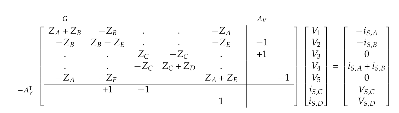
Modified nodal analysis

We add extra unknowns for

• branch currents for voltage sources
• all elements for which it is impossible or inconvenient to write \( i = f(v_1, v_2) \).

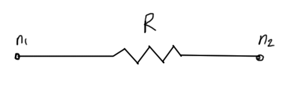
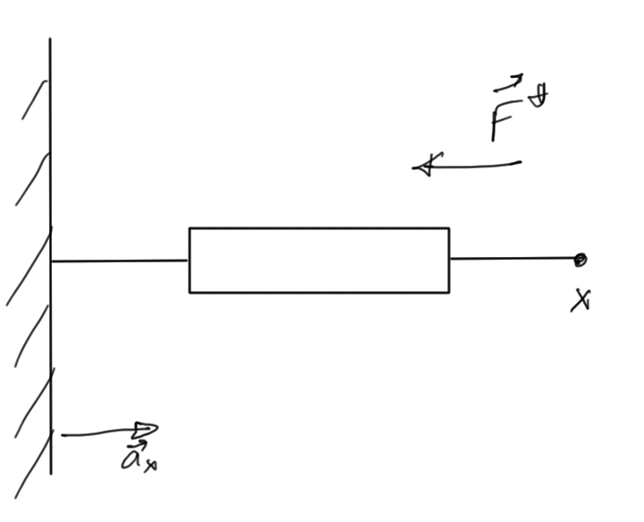
  Imagine, for example, that we have a component illustrated in fig. 1.

  

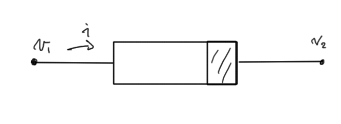
  fig. 1. Variable voltage device

  \begin{equation}\label{eqn:multiphysicsL4:20}
  v_1 – v_2 = 3 i^2
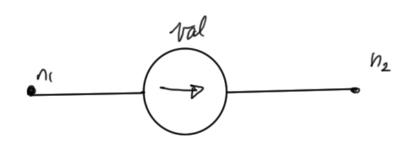
  \end{equation}

• any current which is controlling dependent sources, as in fig. 2.
  

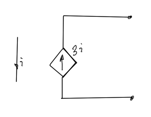
  fig. 2. Current controlled device

• Inductors
  \begin{equation}\label{eqn:multiphysicsL4:40}
  v_1 – v_2 = L \frac{di}{dt}.
  \end{equation}

Solving large systems

We are interested in solving linear systems of the form

\begin{equation}\label{eqn:multiphysicsL4:60}
M \overline{{x}} = \overline{{b}},
\end{equation}

possibly with thousands of elements.

Gaussian elimination

\begin{equation}\label{eqn:multiphysicsL4:80}
\begin{bmatrix}
M_{11} & M_{12} & M_{13} \\
M_{21} & M_{22} & M_{23} \\
M_{31} & M_{32} & M_{33} \\
\end{bmatrix}
\begin{bmatrix}
x_1 \\
x_2 \\
x_3 \\
\end{bmatrix}
=
\begin{bmatrix}
b_1 \\
b_2 \\
b_3 \\
\end{bmatrix}
\end{equation}

It’s claimed for now, to be seen later, that back substitution is the fastest way to arrive at the solution, less computationally complex than completion the diagonalization.

Steps

\begin{equation}\label{eqn:multiphysicsL4:100}
(1) \cdot \frac{M_{21}}{M_{11}} \Rightarrow
\begin{bmatrix}
M_{21} & \frac{M_{21}}{M_{11}} M_{12} & \frac{M_{21}}{M_{11}} M_{13} \\
\end{bmatrix}
\end{equation}

\begin{equation}\label{eqn:multiphysicsL4:120}
(2) \cdot \frac{M_{31}}{M_{11}} \Rightarrow
\begin{bmatrix}
M_{31} & \frac{M_{31}}{M_{11}} M_{32} & \frac{M_{31}}{M_{11}} M_{33} \\
\end{bmatrix}
\end{equation}

This gives

\begin{equation}\label{eqn:multiphysicsL4:140}
\begin{bmatrix}
M_{11} & M_{12} & M_{13} \\
0 & M_{22} – \frac{M_{21}}{ M_{11} } M_{12} & M_{23} – \frac{M_{21}}{M_{11}} M_{13} \\
0 & M_{32} – \frac{M_{31}}{M_{11}} M_{32} & M_{33} – \frac{M_{31}}{M_{11}} M_{33} \\
\end{bmatrix}
\begin{bmatrix}
x_1 \\
x_2 \\
x_3 \\
\end{bmatrix}
=
\begin{bmatrix}
b_1 \\
b_2 – \frac{M_{21}}{M_{11}} b_1 \\
b_3 – \frac{M_{31}}{M_{11}} b_1
\end{bmatrix}.
\end{equation}

Here the \( M_{11} \) element is called the {pivot}. Each of the \(
M_{j1}/M_{11} \) elements is called a {multiplier}. This operation can be written as

\begin{equation}\label{eqn:multiphysicsL4:160}
\begin{bmatrix}
M_{11} & M_{12} & M_{13} \\
0 & M_{22}^{(2)} & M_{23}^{(3)} \\
0 & M_{32}^{(2)} & M_{33}^{(3)} \\
\end{bmatrix}
\begin{bmatrix}
x_1 \\
x_2 \\
x_3 \\
\end{bmatrix}
=
\begin{bmatrix}
b_1 \\
b_2^{(2)} \\
b_3^{(2)} \\
\end{bmatrix}.
\end{equation}

Using \( M_{22}^{(2)} \) as the pivot this time, we form
\begin{equation}\label{eqn:multiphysicsL4:180}
\begin{bmatrix}
M_{11} & M_{12} & M_{13} \\
0 & M_{22}^{(2)} & M_{23}^{(3)} \\
0 & 0 & M_{33}^{(3)} – \frac{M_{32}^{(2)}}{M_{22}^{(2)}} M_{23}^{(2)} \\
\end{bmatrix}
\begin{bmatrix}
x_1 \\
x_2 \\
x_3 \\
\end{bmatrix}
=
\begin{bmatrix}
b_1 \\
b_2 – \frac{M_{21}}{M_{11}} b_1 \\
b_3 – \frac{M_{31}}{M_{11}} b_1
– \frac{M_{32}^{(2)}}{M_{22}^{(2)}} b_{2}^{(2)} \\
\end{bmatrix}.
\end{equation}

LU decomposition

Through Gaussian elimination, we have transformed the system from

\begin{equation}\label{eqn:multiphysicsL4:200}
M x = b
\end{equation}

to
\begin{equation}\label{eqn:multiphysicsL4:220}
U x = y.
\end{equation}

Writing out our Gaussian transformation in the form \( U \overline{{x}} = b \) we have

\begin{equation}\label{eqn:multiphysicsL4:240}
U \overline{{x}} =
\begin{bmatrix}
1 & 0 & 0 \\
-\frac{M_{21}}{M_{11}} & 1 & 0 \\
\frac{M_{32}^{(2)}}{M_{22}^{(2)}}
\frac{M_{21}}{M_{11}}
–
\frac{M_{31}}{M_{11}}
&
–
\frac{M_{32}^{(2)}}{M_{22}^{(2)}}
& 1
\end{bmatrix}
\begin{bmatrix}
b_1 \\
b_2 \\
b_3
\end{bmatrix}.
\end{equation}

We can verify that the operation matrix \( K^{-1} \), where \( K^{-1} U = M \) that takes us to this form is

\begin{equation}\label{eqn:multiphysicsL4:260}
\begin{bmatrix}
1 & 0 & 0 \\
\frac{M_{21}}{M_{11}} & 1 & 0 \\
\frac{M_{31}}{M_{11}} &
\frac{M_{32}^{(2)}}{M_{22}^{(2)}} &
1
\end{bmatrix}
\begin{bmatrix}
U_{11} & U_{12} & U_{13} \\
0 & U_{22} & U_{23} \\
0 & 0 & U_{33} \\
\end{bmatrix}
\overline{{x}} = \overline{{b}}
\end{equation}

Using this {LU} decomposition is generally superior to standard Gaussian elimination, since we can use this for many different \(\overline{{b}}\) vectors using the same amount of work.

Our steps are

\begin{equation}\label{eqn:multiphysicsL4:280}
b
= M x
= L \lr{ U x}
\equiv L y.
\end{equation}

We can now solve \( L y = b \), using substitution for \( y_1 \), then \( y_2 \), and finally \( y_3 \). This is called {forward substitution}.

Finally, we can now solve

\begin{equation}\label{eqn:multiphysicsL4:300}
U x = y,
\end{equation}

using {back substitution}.

Note that we produced the vector \( y \) as a side effect of performing the Gaussian elimination process.