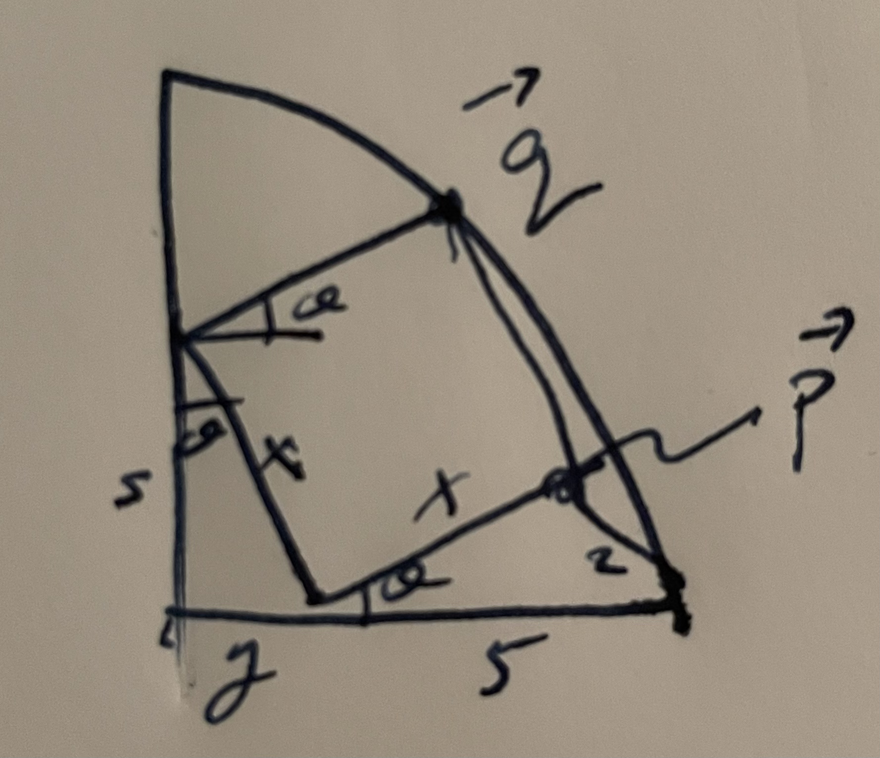
My solution (before numerical reduction), using basic trig and complex numbers, is illustrated in fig. 1.
fig. 1. With complex numbers.
We have
\begin{equation}\label{eqn:squareInCircle:20}
\begin{aligned}
s &= x \cos\theta \\
y &= x \sin\theta \\
p &= y + x e^{i\theta} \\
q &= i s + x e^{i\theta} \\
\Abs{q} &= y + 5 \\
\Abs{p – q} &= 2.
\end{aligned}
\end{equation}
This can be reduced to
\begin{equation}\label{eqn:squareInCircle:40}
\begin{aligned}
\Abs{ x e^{i\theta} – 5 } &= 2 \\
x \Abs{ i \cos\theta + e^{i\theta} } &= x \sin\theta + 5.
\end{aligned}
\end{equation}
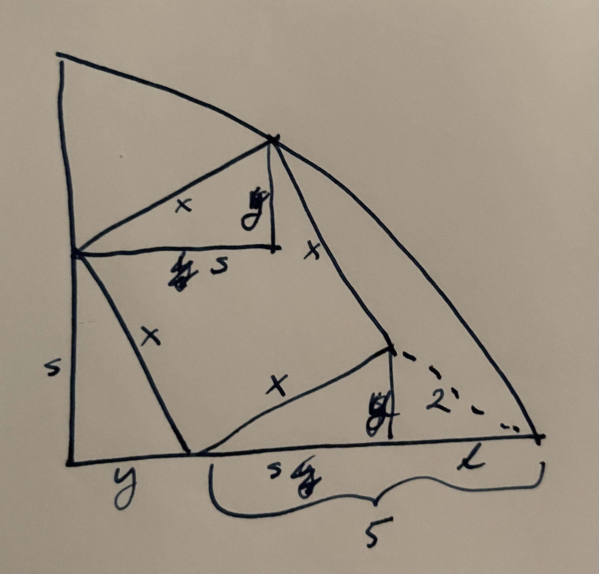
My wife figured out how to do it with just Pythagoras, as illustrated in fig. 2.
fig. 2. With Pythagoras.
\begin{equation}\label{eqn:squareInCircle:60}
\begin{aligned}
\lr{ 5 – s }^2 + y^2 &= 4 \\
\lr{ s + y }^2 + s^2 &= \lr{ y + 5 }^2 \\
x^2 &= s^2 + y^2.
\end{aligned}
\end{equation}
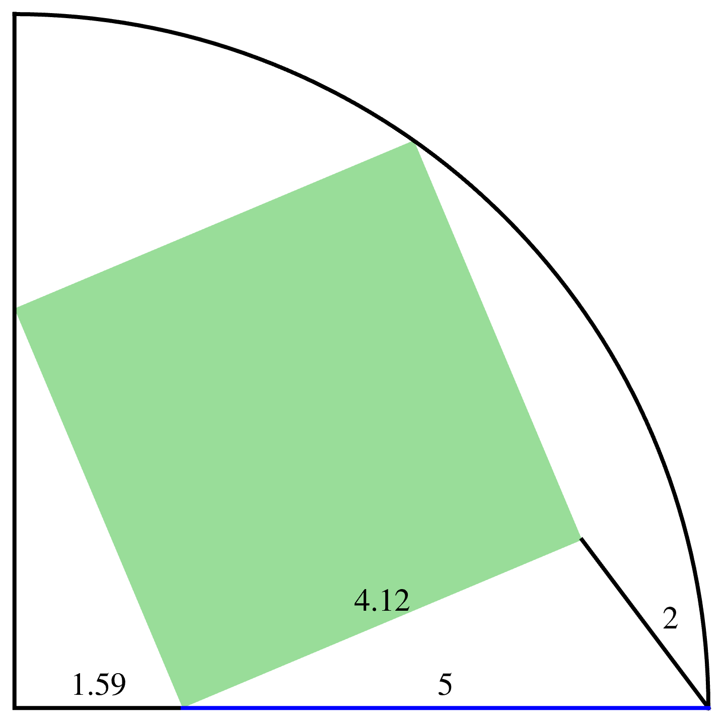
Either way, the numerical solution is 4.12. The geometry looks like fig. 3.
Look below for a wordpress version of this post (and supplementary notes for the video.)
Exact system.
Recall that we can use the wedge product to solve linear systems. For example, assuming that \( \Ba, \Bb \) are not colinear, the system
\begin{equation}\label{eqn:cramersProjection:20}
x \Ba + y \Bb = \Bc,
\end{equation}
if it has a solution, can be solved for \( x \) and \( y \) by wedging with \( \Bb \), and \( \Ba \) respectively.
For example, wedging with \( \Bb \), from the right, gives
\begin{equation}\label{eqn:cramersProjection:40}
x \lr{ \Ba \wedge \Bb } + y \lr{ \Bb \wedge \Bb } = \Bc \wedge \Bb,
\end{equation}
but since \( \Bb \wedge \Bb = 0 \), we are left with
\begin{equation}\label{eqn:cramersProjection:60}
x \lr{ \Ba \wedge \Bb } = \Bc \wedge \Bb,
\end{equation}
and since \( \Ba, \Bb \) are not colinear, which means that \( \Ba \wedge \Bb \ne 0 \), we have
\begin{equation}\label{eqn:cramersProjection:80}
x = \inv{ \Ba \wedge \Bb } \Bc \wedge \Bb.
\end{equation}
Similarly, we can wedge with \( \Ba \) (from the left), to find
\begin{equation}\label{eqn:cramersProjection:100}
y = \inv{ \Ba \wedge \Bb } \Ba \wedge \Bc.
\end{equation}
This works because, if the system has a solution, all the bivectors \( \Ba \wedge \Bb \), \( \Ba \wedge \Bc \), and \( \Bb \wedge \Bc \), are all scalar multiples of each other, so we can just divide the two bivectors, and the results must be scalars.
Cramer’s rule.
Incidentally, observe that for \(\mathbb{R}^2\), this is the “Cramer’s rule” solution to the system, since
\begin{equation}\label{eqn:cramersProjection:180}
\Bx \wedge \By = \begin{vmatrix} \Bx & \By \end{vmatrix} \Be_1 \Be_2,
\end{equation}
where we are treating \( \Bx \) and \( \By \) here as column vectors of the coordinates. This means that, after dividing out the plane pseudoscalar \( \Be_1 \Be_2 \), we have
\begin{equation}\label{eqn:cramersProjection:200}
\begin{aligned}
x
&=
\frac{
\begin{vmatrix}
\Bc & \Bb \\
\end{vmatrix}
}{
\begin{vmatrix}
\Ba & \Bb
\end{vmatrix}
} \\
y
&=
\frac{
\begin{vmatrix}
\Ba & \Bc \\
\end{vmatrix}
}{
\begin{vmatrix}
\Ba & \Bb
\end{vmatrix}
}.
\end{aligned}
\end{equation}
This follows the usual Cramer’s rule proscription, where we form determinants of the coordinates of the spanning vectors, replace either of the original vectors in the numerator with the target vector (depending on which variable we seek), and then take ratios of the two determinants.
Least squares solution, using geometry.
Now, let’s consider the case, where the system \ref{eqn:cramersProjection:20} cannot be solved exactly. Geometrically, the best we can do is to try to solve the related “least squares” problem
\begin{equation}\label{eqn:cramersProjection:120}
x \Ba + y \Bb = \Bc_\parallel,
\end{equation}
where \( \Bc_\parallel \) is the projection of \( \Bc \) onto the plane spanned by \( \Ba, \Bb \). Regardless of the value of \( \Bc \), we can always find a solution to this problem. For example, solving for \( x \), we have
\begin{equation}\label{eqn:cramersProjection:160}
\begin{aligned}
x
&= \inv{ \Ba \wedge \Bb } \Bc_\parallel \wedge \Bb \\
&= \inv{ \Ba \wedge \Bb } \cdot \lr{ \Bc_\parallel \wedge \Bb } \\
&= \inv{ \Ba \wedge \Bb } \cdot \lr{ \Bc \wedge \Bb } – \inv{ \Ba \wedge \Bb } \cdot \lr{ \Bc_\perp \wedge \Bb }.
\end{aligned}
\end{equation}
Let’s look at the second term, which can be written
\begin{equation}\label{eqn:cramersProjection:140}
\begin{aligned}
– \inv{ \Ba \wedge \Bb } \cdot \lr{ \Bc_\perp \wedge \Bb }
&=
– \frac{ \Ba \wedge \Bb }{ \lr{ \Ba \wedge \Bb}^2 } \cdot \lr{ \Bc_\perp \wedge \Bb } \\
&\propto
\lr{ \Ba \wedge \Bb } \cdot \lr{ \Bc_\perp \wedge \Bb } \\
&=
\lr{ \lr{ \Ba \wedge \Bb } \cdot \Bc_\perp } \cdot \Bb \\
&=
\lr{ \Ba \lr{ \Bb \cdot \Bc_\perp} – \Bb \lr{ \Ba \cdot \Bc_\perp} } \cdot \Bb \\
&=
0.
\end{aligned}
\end{equation}
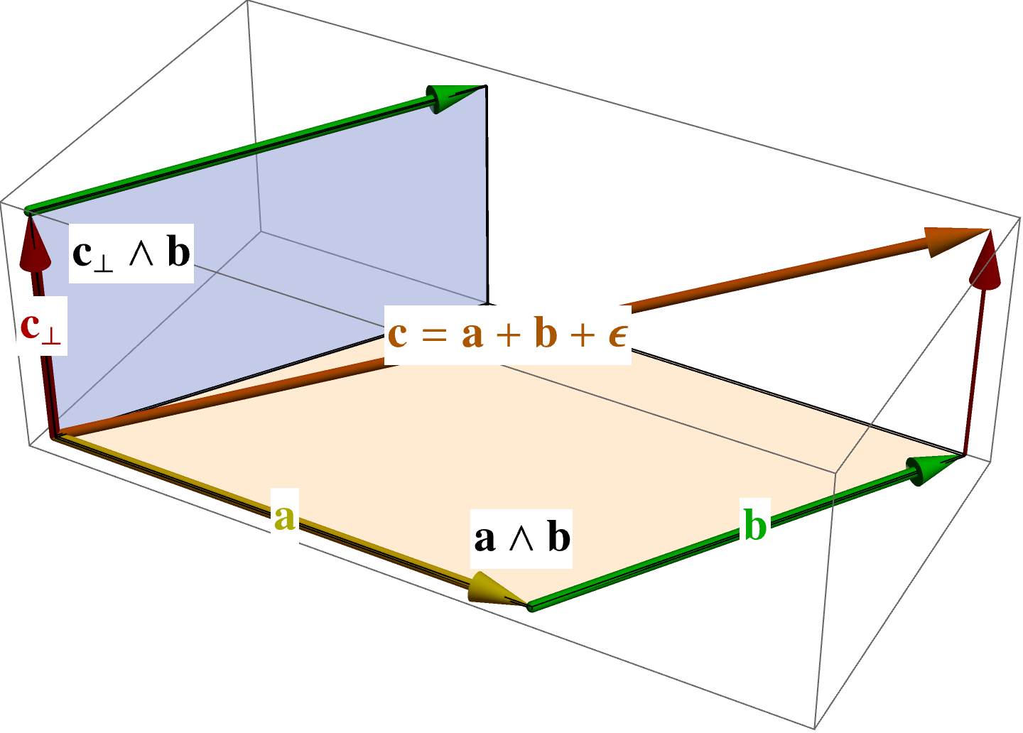
The zero above follows because \( \Bc_\perp \) is perpendicular to both \( \Ba \) and \( \Bb \) by construction. Geometrically, we are trying to dot two perpendicular bivectors, where \( \Bb \) is a common factor of those two bivectors, as illustrated in fig. 1.
fig. 1. Perpendicular bivectors.
We see that our least squares solution, to this two variable linear system problem, is
\begin{equation}\label{eqn:cramersProjection:220}
x = \inv{ \Ba \wedge \Bb } \cdot \lr{ \Bc \wedge \Bb }.
\end{equation}
\begin{equation}\label{eqn:cramersProjection:240}
y = \inv{ \Ba \wedge \Bb } \cdot \lr{ \Ba \wedge \Bc }.
\end{equation}
The interesting thing here is how we have managed to connect the geometric notion of the optimal solution, the equivalent of a least squares solution (which we can compute with the Moore-Penrose inverse, or with an SVD (Singular Value Decomposition)), with the entirely geometric notion of selecting for the portion of the desired solution that lies within the span of the set of input vectors, provided that the spanning vectors for that hyperplane are linearly independent.
Least squares solution, using calculus.
I’ve called the projection solution, a least-squares solution, without full justification. Here’s that justification. We define the usual error function, the squared distance from the target, from our superposition position in the plane
\begin{equation}\label{eqn:cramersProjection:300}
\epsilon = \lr{ \Bc – x \Ba – y \Bb }^2,
\end{equation}
and then take partials with respect to \( x, y \), equating each to zero
\begin{equation}\label{eqn:cramersProjection:320}
\begin{aligned}
0 &= \PD{x}{\epsilon} = 2 \lr{ \Bc – x \Ba – y \Bb } \cdot (-\Ba) \\
0 &= \PD{y}{\epsilon} = 2 \lr{ \Bc – x \Ba – y \Bb } \cdot (-\Bb).
\end{aligned}
\end{equation}
This is a two equation, two unknown system, which can be expressed in matrix form as
\begin{equation}\label{eqn:cramersProjection:340}
\begin{bmatrix}
\Ba^2 & \Ba \cdot \Bb \\
\Ba \cdot \Bb & \Bb^2
\end{bmatrix}
\begin{bmatrix}
x \\
y
\end{bmatrix}
=
\begin{bmatrix}
\Ba \cdot \Bc \\
\Bb \cdot \Bc \\
\end{bmatrix}.
\end{equation}
This has solution
\begin{equation}\label{eqn:cramersProjection:360}
\begin{bmatrix}
x \\
y
\end{bmatrix}
=
\inv{
\begin{vmatrix}
\Ba^2 & \Ba \cdot \Bb \\
\Ba \cdot \Bb & \Bb^2
\end{vmatrix}
}
\begin{bmatrix}
\Bb^2 & -\Ba \cdot \Bb \\
-\Ba \cdot \Bb & \Ba^2
\end{bmatrix}
\begin{bmatrix}
\Ba \cdot \Bc \\
\Bb \cdot \Bc \\
\end{bmatrix}
=
\frac{
\begin{bmatrix}
\Bb^2 \lr{ \Ba \cdot \Bc } – \lr{ \Ba \cdot \Bb} \lr{ \Bb \cdot \Bc } \\
\Ba^2 \lr{ \Bb \cdot \Bc } – \lr{ \Ba \cdot \Bb} \lr{ \Ba \cdot \Bc } \\
\end{bmatrix}
}{
\Ba^2 \Bb^2 – \lr{ \Ba \cdot \Bb }^2
}.
\end{equation}
All of these differences can be expressed as wedge dot products, using the following expansions in reverse
\begin{equation}\label{eqn:cramersProjection:420}
\begin{aligned}
\lr{ \Ba \wedge \Bb } \cdot \lr{ \Bc \wedge \Bd }
&=
\Ba \cdot \lr{ \Bb \cdot \lr{ \Bc \wedge \Bd } } \\
&=
\Ba \cdot \lr{ \lr{\Bb \cdot \Bc} \Bd – \lr{\Bb \cdot \Bd} \Bc } \\
&=
\lr{ \Ba \cdot \Bd } \lr{\Bb \cdot \Bc} – \lr{ \Ba \cdot \Bc }\lr{\Bb \cdot \Bd}.
\end{aligned}
\end{equation}
We find
\begin{equation}\label{eqn:cramersProjection:380}
\begin{aligned}
x
&= \frac{\Bb^2 \lr{ \Ba \cdot \Bc } – \lr{ \Ba \cdot \Bb} \lr{ \Bb \cdot \Bc }}{-\lr{ \Ba \wedge \Bb }^2 } \\
&= \frac{\lr{ \Ba \wedge \Bb } \cdot \lr{ \Bb \wedge \Bc }}{ -\lr{ \Ba \wedge \Bb }^2 } \\
&= \inv{ \Ba \wedge \Bb } \cdot \lr{ \Bc \wedge \Bb },
\end{aligned}
\end{equation}
and
\begin{equation}\label{eqn:cramersProjection:400}
\begin{aligned}
y
&= \frac{\Ba^2 \lr{ \Bb \cdot \Bc } – \lr{ \Ba \cdot \Bb} \lr{ \Ba \cdot \Bc } }{-\lr{ \Ba \wedge \Bb }^2 } \\
&= \frac{- \lr{ \Ba \wedge \Bb } \cdot \lr{ \Ba \wedge \Bc } }{ -\lr{ \Ba \wedge \Bb }^2 } \\
&= \inv{ \Ba \wedge \Bb } \cdot \lr{ \Ba \wedge \Bc }.
\end{aligned}
\end{equation}
Sure enough, we find what was dubbed our least squares solution, which we now know can be written out as a ratio of (dotted) wedge products.
From \ref{eqn:cramersProjection:340}, it wasn’t obvious that the least squares solution would have a structure that was almost Cramer’s rule like, but having solved this problem using geometry alone, we knew to expect that. It was therefore natural to write the results in terms of wedge products factors, and find the simplest statement of the end result. That end result reduces to Cramer’s rule for the \(\mathbb{R}^2\) special case where the system has an exact solution.
We found previously that
\begin{equation}\label{eqn:solarellipse:20}
\mathbf{\hat{r}}’ = \inv{r} \mathbf{\hat{r}} \lr{ \mathbf{\hat{r}} \wedge \Bx’ }.
\end{equation}
Somewhat remarkably, we can use this identity to demonstrate that orbits governed gravitational force are elliptical (or parabolic, or hyperbolic.) This ends up being possible because the angular momentum of the system is a conserved quantity, and this immediately introduces angular momentum into the mix in a fundamental way. In particular,
\begin{equation}\label{eqn:solarellipse:40}
\mathbf{\hat{r}}’ = \inv{m r^2} \mathbf{\hat{r}} L,
\end{equation}
where we define the angular momentum bivector as
\begin{equation}\label{eqn:solarellipse:60}
L = \Bx \wedge \Bp.
\end{equation}
Our gravitational law is
\begin{equation}\label{eqn:solarellipse:80}
m \ddt{\Bv} = – G m M \frac{\mathbf{\hat{r}}}{r^2},
\end{equation}
or
\begin{equation}\label{eqn:solarellipse:100}
-\inv{G M} \ddt{\Bv} = \frac{\mathbf{\hat{r}}}{r^2}.
\end{equation}
Combining the gravitational law with our \( \mathbf{\hat{r}} \) derivative identity, we have
\begin{equation}\label{eqn:solarellipse:120}
\begin{aligned}
\ddt{ \mathbf{\hat{r}} }
&= \inv{m} \frac{\mathbf{\hat{r}}}{r^2} L \\
&= -\inv{G m M} \ddt{\Bv} L \\
&= -\inv{G m M} \lr{ \ddt{(\Bv L)} – \ddt{L} }.
\end{aligned}
\end{equation}
Since angular momentum is a constant of motion of the system, means that
\begin{equation}\label{eqn:solarellipse:140}
\ddt{L} = 0,
\end{equation}
our equation of motion is integratable
\begin{equation}\label{eqn:solarellipse:160}
\ddt{ \mathbf{\hat{r}} } = -\inv{G m M} \ddt{(\Bv L)}.
\end{equation}
Introducing a vector valued integration constant \( -\Be \), we have
\begin{equation}\label{eqn:solarellipse:180}
\mathbf{\hat{r}} = -\inv{G m M} \Bv L – \Be.
\end{equation}
We’ve transformed our second order differential equation to a first order equation, one that does not look easy to integrate one more time. Luckily, we do not have to integrate, and can partially solve this algebraically, enough to describe the orbit in a compact fashion.
Before trying that, it’s worth quickly demonstrating that this equation is not a multivector equation, but a vector equation, since the multivector \( \Bv L \) is, in fact, vector valued.
\begin{equation}\label{eqn:solarellipse:200}
\begin{aligned}
\Bv L
&= \Bv \lr{ \Bx \wedge (m \Bv) } \\
&\propto \mathbf{\hat{v}} \lr{ \mathbf{\hat{r}} \wedge \mathbf{\hat{v}} } \\
&= \mathbf{\hat{v}} \cdot \lr{ \mathbf{\hat{r}} \wedge \mathbf{\hat{v}} } + \mathbf{\hat{v}} \wedge \lr{ \mathbf{\hat{r}} \wedge \mathbf{\hat{v}} } \\
&= \mathbf{\hat{v}} \cdot \lr{ \mathbf{\hat{r}} \wedge \mathbf{\hat{v}} } \\
&= \lr{ \mathbf{\hat{v}} \cdot \mathbf{\hat{r}} } \mathbf{\hat{v}} – \mathbf{\hat{r}},
\end{aligned}
\end{equation}
which is a vector (i.e.: a vector that is directed along the portion of \( \Bx \) that is perpendicular to \( \Bv \).)
We can reduce \ref{eqn:solarellipse:180} to a scalar equation by dotting with \( \Bx = r \mathbf{\hat{r}} \), leaving
\begin{equation}\label{eqn:solarellipse:220}
\begin{aligned}
r
&= -\inv{G m M} \gpgradezero{ \Bx \Bv L } – \Bx \cdot \Be \\
&= -\inv{G m^2 M} \gpgradezero{ \Bx \Bp L } – \Bx \cdot \Be \\
&= -\inv{G m^2 M} \gpgradezero{ \lr{ \Bx \cdot \Bp + L } L } – \Bx \cdot \Be \\
&= -\inv{G m^2 M} L^2 – \Bx \cdot \Be,
\end{aligned}
\end{equation}
or
\begin{equation}\label{eqn:solarellipse:240}
r = -\frac{L^2}{G M m^2} – r e \cos\theta,
\end{equation}
or
\begin{equation}\label{eqn:solarellipse:260}
r \lr{ 1 + e \cos\theta } = -\frac{L^2}{G M m^2}.
\end{equation}
Observe that the RHS constant is a positive constant, since \( L^2 \le 0 \). This has the structure of a conic section, if we write
\begin{equation}\label{eqn:solarellipse:280}
-\frac{L^2}{G M m^2} = e d.
\end{equation}
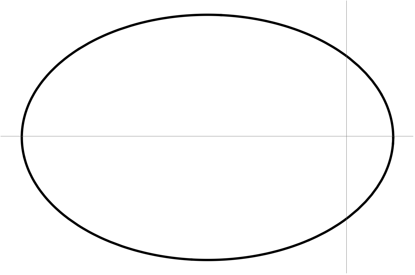
This is an ellipse, for \( e \in [0,1) \), a parabola for \( e = 1 \), and hyperbola for \( e > 1 \) ([1] theorem 10.3.1).
fig. 1. Ellipse with e = 0.75
In fig. 1 is a plot with \( e = 0.75 \) (changing \( d \) doesn’t change the shape of the figure, just the size.)
References
[1] S.L. Salas and E. Hille. Calculus: one and several variables. Wiley New York, 1990.
We found the form of the unit vector derivatives in both cases.
\begin{equation}\label{eqn:radialderivatives:20}
\Bx = r \mathbf{\hat{r}},
\end{equation}
leaving the angular dependence of \( \mathbf{\hat{r}} \) unspecified. We want to find both \( \Bv = \Bx’ \) and \( \mathbf{\hat{r}}’\).
Derivatives.
Lemma 1.1: Radial length derivative.
The derivative of a spherical length \( r \) can be expressed as
\begin{equation*}
\frac{dr}{dt} = \mathbf{\hat{r}} \cdot \frac{d\Bx}{dt}.
\end{equation*}
Start proof:
We write \( r^2 = \Bx \cdot \Bx \), and take derivatives of both sides, to find
\begin{equation}\label{eqn:radialderivatives:60}
2 r \frac{dr}{dt} = 2 \Bx \cdot \frac{d\Bx}{dt},
\end{equation}
or
\begin{equation}\label{eqn:radialderivatives:80}
\frac{dr}{dt} = \frac{\Bx}{r} \cdot \frac{d\Bx}{dt} = \mathbf{\hat{r}} \cdot \frac{d\Bx}{dt}.
\end{equation}
End proof.
Application of the chain rule to \ref{eqn:radialderivatives:20} is straightforward
\begin{equation}\label{eqn:radialderivatives:100}
\Bx’ = r’ \mathbf{\hat{r}} + r \mathbf{\hat{r}}’,
\end{equation}
but we don’t know the form for \( \mathbf{\hat{r}}’ \). We could proceed with a niave expansion of
\begin{equation}\label{eqn:radialderivatives:120}
\frac{d}{dt} \lr{ \frac{\Bx}{r} },
\end{equation}
but we can be sneaky, and perform a projective and rejective split of \( \Bx’ \) with respect to \( \mathbf{\hat{r}} \). That is
\begin{equation}\label{eqn:radialderivatives:140}
\begin{aligned}
\Bx’
&= \mathbf{\hat{r}} \mathbf{\hat{r}} \Bx’ \\
&= \mathbf{\hat{r}} \lr{ \mathbf{\hat{r}} \Bx’ } \\
&= \mathbf{\hat{r}} \lr{ \mathbf{\hat{r}} \cdot \Bx’ + \mathbf{\hat{r}} \wedge \Bx’} \\
&= \mathbf{\hat{r}} \lr{ r’ + \mathbf{\hat{r}} \wedge \Bx’}.
\end{aligned}
\end{equation}
We used our lemma in the last step above, and after distribution, find
\begin{equation}\label{eqn:radialderivatives:160}
\Bx’ = r’ \mathbf{\hat{r}} + \mathbf{\hat{r}} \lr{ \mathbf{\hat{r}} \wedge \Bx’ }.
\end{equation}
Comparing to \ref{eqn:radialderivatives:100}, we see that
\begin{equation}\label{eqn:radialderivatives:180}
r \mathbf{\hat{r}}’ = \mathbf{\hat{r}} \lr{ \mathbf{\hat{r}} \wedge \Bx’ }.
\end{equation}
We see that the radial unit vector derivative is proportional to the rejection of \( \mathbf{\hat{r}} \) from \( \Bx’ \)
\begin{equation}\label{eqn:radialderivatives:200}
\mathbf{\hat{r}}’ = \inv{r} \mathrm{Rej}_{\mathbf{\hat{r}}}(\Bx’) = \inv{r^3} \Bx \lr{ \Bx \wedge \Bx’ }.
\end{equation}
The vector \( \mathbf{\hat{r}}’ \) is perpendicular to \( \mathbf{\hat{r}} \) for any parameterization of it’s orientation, or in symbols
\begin{equation}\label{eqn:radialderivatives:220}
\mathbf{\hat{r}} \cdot \mathbf{\hat{r}}’ = 0.
\end{equation}
We saw this for the circular and spherical parameterizations, and see now that this also holds more generally.
Angular momentum.
Let’s now write out the momentum \( \Bp = m \Bv \) for a point particle with mass \( m \), and determine the kinetic energy \( m \Bv^2/2 = \Bp^2/2m \) for that particle.
The momentum is
\begin{equation}\label{eqn:radialderivatives:320}
\begin{aligned}
\Bp
&= m r’ \mathbf{\hat{r}} + m \mathbf{\hat{r}} \lr{ \mathbf{\hat{r}} \wedge \Bv } \\
&= m r’ \mathbf{\hat{r}} + \inv{r} \mathbf{\hat{r}} \lr{ \Br \wedge \Bp }.
\end{aligned}
\end{equation}
Observe that \( p_r = m r’ \) is the radial component of the momentum. It is natural to introduce a bivector valued angular momentum operator
\begin{equation}\label{eqn:radialderivatives:340}
L = \Br \wedge \Bp,
\end{equation}
splitting the momentum into a component that is strictly radial and a component that lies purely on the surface of a spherical surface in momentum space. That is
\begin{equation}\label{eqn:radialderivatives:360}
\Bp = p_r \mathbf{\hat{r}} + \inv{r} \mathbf{\hat{r}} L.
\end{equation}
Making use of the fact that \( \mathbf{\hat{r}} \) and \( \mathrm{Rej}_{\mathbf{\hat{r}}}(\Bx’) \) are perpendicular (so there are no cross terms when we square the momentum), the
kinetic energy is
\begin{equation}\label{eqn:radialderivatives:380}
\begin{aligned}
\inv{2m} \Bp^2
&= \inv{2m} \lr{ p_r \mathbf{\hat{r}} + \inv{r} \mathbf{\hat{r}} L }^2 \\
&= \inv{2m} p_r^2 + \inv{2 m r^2 } \mathbf{\hat{r}} L \mathbf{\hat{r}} L \\
&= \inv{2m} p_r^2 – \inv{2 m r^2 } \mathbf{\hat{r}} L^2 \mathbf{\hat{r}} \\
&= \inv{2m} p_r^2 – \inv{2 m r^2 } L^2 \mathbf{\hat{r}}^2,
\end{aligned}
\end{equation}
where we’ve used the anticommutative nature of \( \mathbf{\hat{r}} \) and \( L \) (i.e.: a sign swap is needed to swap them), and used the fact that \( L^2 \) is a scalar, allowing us to commute \( \mathbf{\hat{r}} \) with \( L^2 \). This leaves us with
\begin{equation}\label{eqn:radialderivatives:400}
E = \inv{2m} \Bp^2 = \inv{2m} p_r^2 – \inv{2 m r^2 } L^2.
\end{equation}
Observe that both the radial momentum term and the angular momentum term are both strictly postive, since \( L \) is a bivector and \( L^2 \le 0 \).
Problems.
Problem:
Find \ref{eqn:radialderivatives:200} without being sneaky.
Show that \ref{eqn:radialderivatives:200} can be expressed as a triple vector cross product
\begin{equation}\label{eqn:radialderivatives:230}
\mathbf{\hat{r}}’ = \inv{r^3} \lr{ \Bx \cross \Bx’ } \cross \Bx,
\end{equation}
Answer
While this may be familiar from elementary calculus, such as in [1], we can show follows easily from our GA result
\begin{equation}\label{eqn:radialderivatives:300}
\begin{aligned}
\mathbf{\hat{r}}’
&= \inv{r} \mathbf{\hat{r}} \lr{ \mathbf{\hat{r}} \wedge \Bx’ } \\
&= \inv{r} \gpgradeone{ \mathbf{\hat{r}} \lr{ \mathbf{\hat{r}} \wedge \Bx’ } } \\
&= \inv{r} \gpgradeone{ \mathbf{\hat{r}} I \lr{ \mathbf{\hat{r}} \cross \Bx’ } } \\
&= \inv{r} \gpgradeone{ I \lr{ \mathbf{\hat{r}} \cdot \lr{ \mathbf{\hat{r}} \cross \Bx’ } + \mathbf{\hat{r}} \wedge \lr{ \mathbf{\hat{r}} \cross \Bx’ } } } \\
&= \inv{r} \gpgradeone{ I^2 \mathbf{\hat{r}} \cross \lr{ \mathbf{\hat{r}} \cross \Bx’ } } \\
&= \inv{r} \lr{ \mathbf{\hat{r}} \cross \Bx’ } \cross \mathbf{\hat{r}}.
\end{aligned}
\end{equation}
References
[1] S.L. Salas and E. Hille. Calculus: one and several variables. Wiley New York, 1990.
We then compute kinetic energy in this representation, and show how a bivector-valued angular momentum \( L = \mathbf{x} \wedge \mathbf{p} \), falls naturally from that computation, where we have
Prerequisites: calculus (derivatives and chain rule), and geometric algebra basics (vector multiplication, commutation relationships for vectors and bivectors in a plane, wedge and cross product equivalencies, …)
Errata: at around 4:12 I used \( \mathbf{r} \) instead of \( \mathbf{x} \), then kept doing so every time after that when the value for \( L \) was stated.