[Click here for a PDF version of this post]
Motivation.
A fun application of both Green’s functions and geometric algebra is to show how the Cauchy integral equation can be expressed in terms of the Green’s function for the 2D gradient. This is covered, almost as an aside, in [1]. I found that treatment a bit hard to understand, so I am going to work through it here at my own pace.
Complex numbers in geometric algebra.
Anybody who has studied geometric algebra is likely familiar with a variety of ways to construct complex numbers from geometric objects. For example, complex numbers can be constructed for any plane. If \( \Be_1, \Be_2 \) is a pair of orthonormal vectors for some plane in \(\mathbb{R}^N\), then any vector in that plane has the form
\begin{equation}\label{eqn:residueGreens:20}
\Bf = \Be_1 u + \Be_2 v,
\end{equation}
has an associated complex representation, by simply multiplying that vector one of those basis vectors. For example, if we pre-multiply \( \Bf \) by \( \Be_1 \), forming
\begin{equation}\label{eqn:residueGreens:40}
\begin{aligned}
z
&= \Be_1 \Bf \\
&= \Be_1 \lr{ \Be_1 u + \Be_2 v } \\
&= u + \Be_1 \Be_2 v.
\end{aligned}
\end{equation}
We may identify the unit bivector \( \Be_1 \Be_2 \) as an imaginary, designed by \( i \), since it has the expected behavior
\begin{equation}\label{eqn:residueGreens:60}
\begin{aligned}
i^2 &=
\lr{\Be_1 \Be_2}^2 \\
&=
\lr{\Be_1 \Be_2}
\lr{\Be_1 \Be_2} \\
&=
\Be_1 \lr{\Be_2
\Be_1} \Be_2 \\
&=
-\Be_1 \lr{\Be_1
\Be_2} \Be_2 \\
&=
-\lr{\Be_1 \Be_1}
\lr{\Be_2 \Be_2} \\
&=
-1.
\end{aligned}
\end{equation}
Complex numbers are seen to be isomorphic to even grade multivectors in a planar subspace. The imaginary is the grade-two pseudoscalar, and geometrically is an oriented unit area (bivector.)
Cauchy-equations in terms of the gradient.
It is natural to wonder about the geometric algebra equivalents of various complex-number relationships and identities. Of particular interest for this discussion is the geometric algebra equivalent of the Cauchy equations that specify required conditions for a function to be differentiable.
If a complex function \( f(z) = u(z) + i v(z) \) is differentiable, then we must be able to find the limit of
\begin{equation}\label{eqn:residueGreens:80}
\frac{\Delta f(z_0)}{\Delta z} = \frac{f(z_0 + h) – f(z_0)}{h},
\end{equation}
for any complex \( h \rightarrow 0 \), for any possible trajectory of \( z_0 + h \) toward \( z_0 \). In particular, for real \( h = \epsilon \),
\begin{equation}\label{eqn:residueGreens:100}
\lim_{\epsilon \rightarrow 0} \frac{u(x_0 + \epsilon, y_0) + i v(x_0 + \epsilon, y_0) – u(x_0, y_0) – i v(x_0, y_0)}{\epsilon}
=
\PD{x}{u(z_0)} + i \PD{x}{v(z_0)},
\end{equation}
and for imaginary \( h = i \epsilon \)
\begin{equation}\label{eqn:residueGreens:120}
\lim_{\epsilon \rightarrow 0} \frac{u(x_0, y_0 + \epsilon) + i v(x_0, y_0 + \epsilon) – u(x_0, y_0) – i v(x_0, y_0)}{i \epsilon}
=
-i\lr{ \PD{y}{u(z_0)} + i \PD{y}{v(z_0)} }.
\end{equation}
Equating real and imaginary parts, we see that existence of the derivative requires
\begin{equation}\label{eqn:residueGreens:140}
\begin{aligned}
\PD{x}{u} &= \PD{y}{v} \\
\PD{x}{v} &= -\PD{y}{u}.
\end{aligned}
\end{equation}
These are the Cauchy equations. When the derivative exists in a given neighbourhood, we say that the function is analytic in that region. If we use a bivector interpretation of the imaginary, with \( i = \Be_1 \Be_2 \), the Cauchy equations are also satisfied if the gradient of the complex function is zero, since
\begin{equation}\label{eqn:residueGreens:160}
\begin{aligned}
\spacegrad f
&=
\lr{ \Be_1 \partial_x + \Be_2 \partial_y } \lr{ u + \Be_1 \Be_2 v } \\
&=
\Be_1 \lr{ \partial_x u – \partial_y v } + \Be_2 \lr{ \partial_y u + \partial_x v }.
\end{aligned}
\end{equation}
We see that the geometric algebra equivalent of the Cauchy equations is simply
\begin{equation}\label{eqn:residueGreens:200}
\spacegrad f = 0.
\end{equation}
Roughly speaking, we may say that a function is analytic in a region, if the Cauchy equations are satisfied, or the gradient is zero, in a neighbourhood of all points in that region.
A special case of the fundamental theorem of geometric calculus.
Given an even grade multivector \( \psi \in \mathbb{R}^2 \) (i.e.: a complex number), we can show that
\begin{equation}\label{eqn:residueGreens:220}
\int_A \spacegrad \psi d^2\Bx = \oint_{\partial A} d\Bx \psi.
\end{equation}
Let’s get an idea why this works by expanding the area integral for a rectangular parameterization
\begin{equation}\label{eqn:residueGreens:240}
\begin{aligned}
\int_A \spacegrad \psi d^2\Bx
&=
\int_A \lr{ \Be_1 \partial_1 + \Be_2 \partial_2 } \psi I dx dy \\
&=
\int \Be_1 I dy \evalrange{\psi}{x_0}{x_1}
+
\int \Be_2 I dx \evalrange{\psi}{y_0}{y_1} \\
&=
\int \Be_2 dy \evalrange{\psi}{x_0}{x_1}
–
\int \Be_1 dx \evalrange{\psi}{y_0}{y_1} \\
&=
\int d\By \evalrange{\psi}{x_0}{x_1}
–
\int d\Bx \evalrange{\psi}{y_0}{y_1}.
\end{aligned}
\end{equation}
We took advantage of the fact that the \(\mathbb{R}^2\) pseudoscalar commutes with \( \psi \). The end result, is illustrated in fig. 1, shows pictorially that the remaining integral is an oriented line integral.

fig. 1. Oriented multivector line integral.
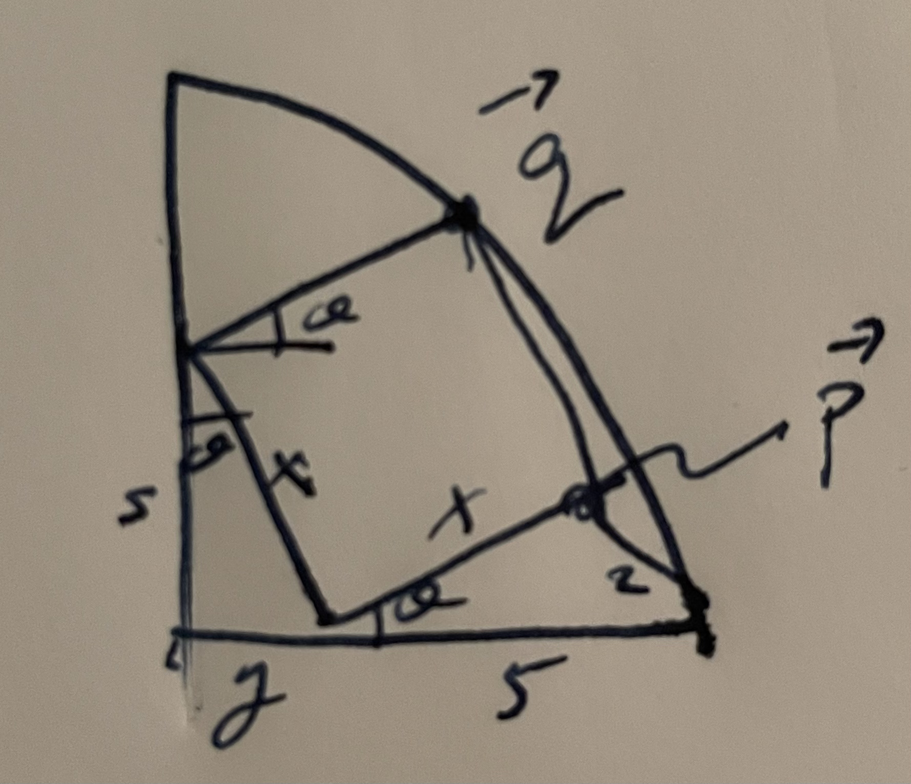
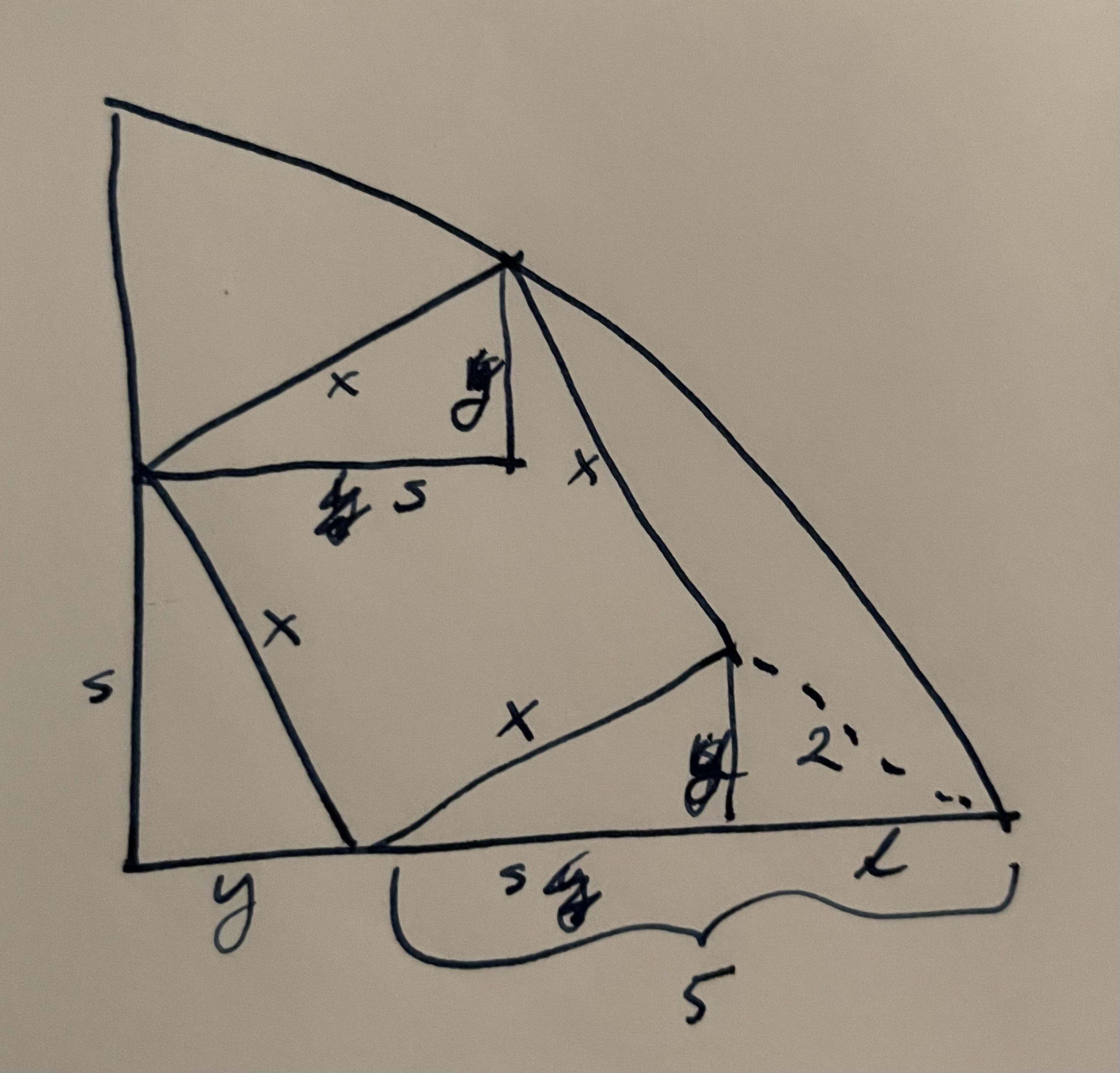
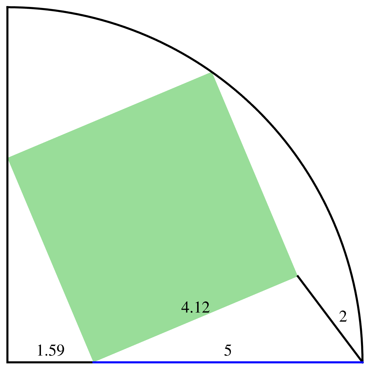
If we want to approximate a more general area, we may do so with additional tiles, as illustrated in fig. 2. We may evaluate the area integral using the line integral over just the exterior boundary using such a tiling, as any overlapping opposing boundary contributions cancel exactly.

fig. 2. A crude circular tiling approximation.
The reason that this is interesting is that it allows us to re-express a complex integral as a corresponding multivector area integral. With \( d\Bx = \Be_1 dz \), we have
\begin{equation}\label{eqn:residueGreens:260}
\oint dz\, \psi = \Be_1 \int \spacegrad \psi d^2\Bx.
\end{equation}
The Cauchy kernel as a Green’s function.
We’ve previously derived the Green’s function for the 2D Laplacian, and found
\begin{equation}\label{eqn:residueGreens:280}
\tilde{G}(\Bx, \Bx’) = \inv{2\pi} \ln \Abs{\lr{\Bx – \Bx’}},
\end{equation}
which satisfies
\begin{equation}\label{eqn:residueGreens:300}
\delta^2(\Bx – \Bx’) = \spacegrad^2 \tilde{G}(\Bx, \Bx’) = \spacegrad \lr{ \spacegrad \tilde{G}(\Bx, \Bx’) }.
\end{equation}
This means that \( G(\Bx, \Bx’) = \spacegrad \tilde{G}(\Bx, \Bx’) \) is the Green’s function for the gradient. That Green’s function is
\begin{equation}\label{eqn:residueGreens:320}
\begin{aligned}
G(\Bx, \Ba)
&= \inv{2 \pi} \frac{\spacegrad \Abs{\Bx – \Ba}}{\Abs{\Bx – \Ba}} \\
&= \inv{2 \pi} \frac{\Bx – \Ba}{\Abs{\Bx – \Ba}^2}.
\end{aligned}
\end{equation}
We may cast this Green’s function into complex form with \( z = \Be_1 \Bx, a = \Be_1 \Ba \). In particular
\begin{equation}\label{eqn:residueGreens:340}
\begin{aligned}
\inv{z – a}
&=
\frac{(z – a)^\conj}{\Abs{z – a}^2} \\
&=
\frac{(z – a)^\conj}{\Abs{z – a}^2} \\
&=
\frac{\Bx – \Ba}{\Abs{\Bx – \Ba}^2} \Be_1 \\
&=
2 \pi G(\Bx, \Ba) \Be_1.
\end{aligned}
\end{equation}
Cauchy’s integral.
With
\begin{equation}\label{eqn:residueGreens:360}
\psi = \frac{f(z)}{z – a},
\end{equation}
using \ref{eqn:residueGreens:260}, we can now evaluate
\begin{equation}\label{eqn:residueGreens:265}
\begin{aligned}
\oint dz\, \frac{f(z)}{z – a}
&= \Be_1 \int \spacegrad \frac{f(z)}{z – a} d^2\Bx \\
&= \Be_1 \int \lr{ \frac{\spacegrad f(z)}{z – a} + \lr{ \spacegrad \inv{z – a}} f(z) } I dA \\
&= \Be_1 \int f(z) \spacegrad 2 \pi G(\Bx – \Ba) \Be_1 I dA \\
&= 2 \pi \Be_1 \int \delta^2(\Bx – \Ba) \Be_1 f(\Bx) I dA \\
&= 2 \pi \Be_1^2 f(\Ba) I \\
&= 2 \pi I f(a),
\end{aligned}
\end{equation}
where we’ve made use of the analytic condition \( \spacegrad f = 0 \), and the fact that \( f \) and \( 1/(z-a) \), both even multivectors, commute.
The Cauchy integral equation
\begin{equation}\label{eqn:residueGreens:380}
f(a) = \inv{2 \pi I} \oint dz\, \frac{f(z)}{z – a},
\end{equation}
falls out naturally. This sort of residue calculation always seemed a bit miraculous. By introducing a geometric algebra encoding of complex numbers, we get a new and interesting interpretation. In particular,
- the imaginary factor in the geometric algebra formulation of this identity is an oriented unit area coming directly from the area element,
- the factor of \( 2 \pi \) comes directly from the Green’s function for the gradient,
- the fact that this particular form of integral picks up only the contribution at the point \( z = a \) is no longer mysterious seeming. This is directly due to delta-function filtering.
Also, if we are looking for an understanding of how to generalize the Cauchy equation to more general multivector functions, we now also have a good clue how that would be done.
References
[1] C. Doran and A.N. Lasenby. Geometric algebra for physicists. Cambridge University Press New York, Cambridge, UK, 1st edition, 2003.