Month: November 2016

Political correctness

November 24, 2016 Incoherent ramblings , , , , , , , ,

I saw an article on facebook about some recent idiocy at Queen’s university.

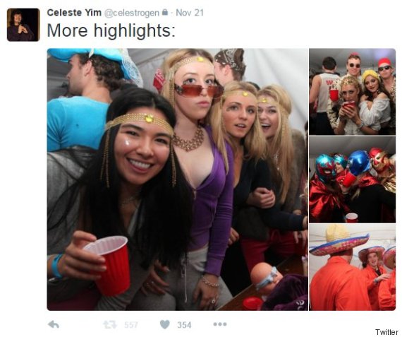
The idiocy isn’t what is being dubbed a racist party, but the fact that a costume party is dubbed racist.

A comment on this (Leon) that I thought summed things up nicely was:

“It is people who criticize a bunch of kids dressing as racists who make incidents of real racism greatly diminished.”

There is an alarming trend of perverting language in the political correct circles that is mystifying

  • A kiss without a contract, triple signed and witnessed, is now being called rape, or it’s seeming legal equivalent “sexual assault”.  There are concent posters all over UofT that outline the legalistic contracting required for sexuality in this PC age.  I was too inhibited when I was an undergrad to have had much sexual activity, but I’m glad that I’m not an undergrad now subject to the current guidelines.  It’s definitely not okay to take advantage of somebody who is drunk, but this has been flipped on its head.  Sex after consentual codrunkenness now appears to be sexual assult in some places.
  • Failing to use the “correct” gendered pronoun is now “hate speech”, and is perceived as, or at least mislabelled as, explicit violence.  I’m a firm believer that people should have complete freedom to engage in hate speech or discrimination of any sort.  Let people dig themselves their own social graves instead of trying to legislate speech.
  • Costume parties, even at halloween, are now being mislabelled racist.  Attempting to point that out at some PC universities resulted in so much PC backlash that resignations followed.

I keep hearing about instance after instance of such events.  It seems like most of the people who are pushing the political correctness agenda really desperately need dictionaries.  Just because you can label two things as identical, doesn’t mean that they are.  A perfect example of this is the use of “sexual assault” now instead of rape.  The two are now identified as identical, even though sexual assault is a much broader term that includes groping.

There was lots in the recent US election media circus about how Trump’s bragging of pussy grabbing and aggressive kissing, acts that were facilitated by stardom.  One of the debate moderators explicitly called that sexual assault.  I don’t like the phrase sexual assault, because it is ambiguous, and has connotations of rape, while not necessarily being rape.  It seems to be a phrase designed to have the emotional impact of rape, while being something lesser.

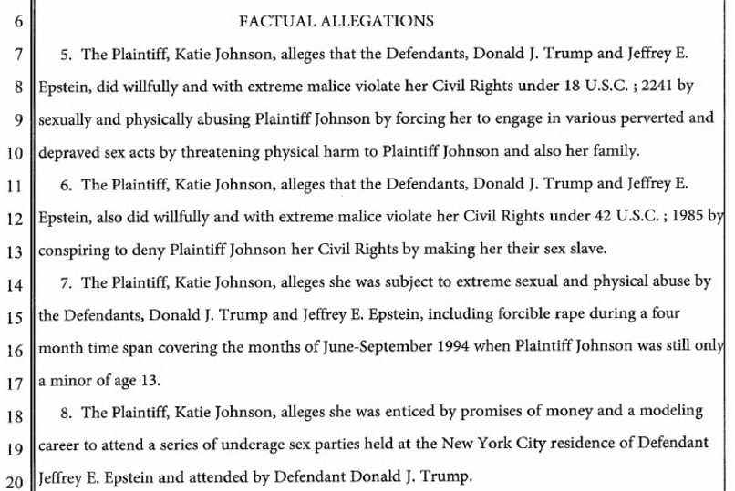
Whether or not that Trump was bragging about sexual assault is probably dependent on state law.  Ambiguous language identifies unequal events with the same weight, and seems to be a characteristic of political correct speech and activism.  For example, calling pussy grabbing rape would be an obvious example of the misuse of language.  That’s why PC correct speech uses sexual assault instead.  A side effect of such PC correct speech is that actual rape, a horribly abusive event, is trivialized.  The irony in the Trump case was that the media could have focused on actual rape.  For example, Trump and his pedophile buddy Jeffrey Epstein, are codefendents in an actual rape case (which I understand has now unfortunately been dropped due to technicalities).  Characteristic of many of the charges laid against Epstein, this one is also of a child, in this case a 13 year old.

Of his buddy Epstein Trump said

“I’ve known Jeff for fifteen years. Terrific guy. He’s a lot of fun to be with. It is even said that he likes beautiful women as much as I do, and many of them are on the younger side.”

It remains to see if Trump is a sexual predator on par with Bill Clinton.  My gut feeling why pussy grabbing got so much attention, but Trump’s case with Epstein did not was because Bill is also a good friend of Epstein, and had been down to Epstein’s pedophile island many times.  Raising attention to that would have distracted from Hillary’s campaign (perhaps even raised the issue that she’d also “partied” there, in ways currently unspecified).

I digress.

How can political correctness be combatted?  One way is calling out explicit misuse of language.  Be very careful to use accurate words, and not to conflate things in order to push an agenda.

Because the political correctness movement is anti-intellectual, I suspect that purely linguistic techniques to fighting it are doomed.  Are there active social techniques that would be effective?

I came up with one idea that I amused myself with.  Perhaps it is time to start hosting some explicitly politically incorrect parties, just to push back.  Imagine a Halloween party that you are not allowed into, unless you are offending some minority group.  Suggested costume ideas include Hilter, blackface, transvestites or red-indians.  If you aren’t insulting somebody, then you can’t come in.  If you don’t think that Hilter is offensive enough, perhaps the host would allow you in if you dressed as some other psychopathic killer like Kissinger or Churchill, but that risks turning the party into an political party instead of an anti-PC party.  Costume prize adjudication would be biased against those that are in a visible minority group, so you should get extra points if you are a cis gendered white male.  Bonus points to the hosts of the party should they hold it on a university campus.

Fresnel angular sum and difference formulas

November 22, 2016 math and physics play , ,

[Click here for a PDF of this post with nicer formatting]

In [1] are some sum and angle difference formulations for the Fresnel formulas given a \( \mu_1 = \mu_2 \) constraint. The proof of these trig Fresnel equations is left to an exercise, and will be derived here.

We need a couple trig identities to start with.

\begin{equation}\label{eqn:fresnelSumAndDifferenceAngleFormulas:20}
\begin{aligned}
\sin(a + b)
&=
\textrm{Im}\lr{ e^{j(a + b)} } \\
&=
\textrm{Im}\lr{
e^{ja} e^{+ jb}
} \\
&=
\textrm{Im}\lr{
(\cos a + j \sin a) (\cos b + j \sin b)
} \\
&=
\sin a \cos b + \cos a \sin b.
\end{aligned}
\end{equation}

Allowing for both signs we have

\begin{equation}\label{eqn:fresnelSumAndDifferenceAngleFormulas:240}
\begin{aligned}
\sin(a + b) &= \sin a \cos b + \cos a \sin b \\
\sin(a – b) &= \sin a \cos b – \cos a \sin b.
\end{aligned}
\end{equation}

The mixed sine and cosine product can be expressed as a sum of sines

\begin{equation}\label{eqn:fresnelSumAndDifferenceAngleFormulas:40}
2 \sin a \cos b = \sin(a + b) + \sin(a – b).
\end{equation}

With \( 2 x = a + b, 2 y = a – b \), or \( a = x + y, b = x – y \), we find

\begin{equation}\label{eqn:fresnelSumAndDifferenceAngleFormulas:60}
\begin{aligned}
2 \sin(x + y) \cos (x – y) &= \sin( 2 x ) + \sin( 2 y ) \\
2 \sin(x – y) \cos (x + y) &= \sin( 2 x ) – \sin( 2 y ).
\end{aligned}
\end{equation}

Returning to the problem. When \( \mu_1 = \mu_2 \) the Fresnel equations were found to be

\begin{equation}\label{eqn:fresnelSumAndDifferenceAngleFormulas:100}
\begin{aligned}
r^{\textrm{TE}} &= \frac { n_1 \cos\theta_i – n_2 \cos\theta_t } { n_1 \cos\theta_i + n_2 \cos\theta_t } \\
r^{\textrm{TM}} &= \frac{n_2 \cos\theta_i – n_1 \cos\theta_t }{ n_2 \cos\theta_i + n_1 \cos\theta_t } \\
t^{\textrm{TE}} &= \frac{ 2 n_1 \cos\theta_i } { n_1 \cos\theta_i + n_2 \cos\theta_t } \\
t^{\textrm{TM}} &= \frac{2 n_1 \cos\theta_i }{ n_2 \cos\theta_i + n_1 \cos\theta_t }.
\end{aligned}
\end{equation}

Using Snell’s law, one of \( n_1, n_2 \) can be eliminated, for example

\begin{equation}\label{eqn:fresnelSumAndDifferenceAngleFormulas:120}
n_1 = n_2 \frac{\sin \theta_t}{\sin\theta_i}.
\end{equation}

Inserting this and proceeding with the application of the trig identities above, we have

\begin{equation}\label{eqn:fresnelSumAndDifferenceAngleFormulas:160}
\begin{aligned}
r^{\textrm{TE}}
&= \frac { n_2 \frac{\sin\theta_t}{\sin\theta_i} \cos\theta_i – n_2 \cos\theta_t } { n_2 \frac{\sin\theta_t}{\sin\theta_i} \cos\theta_i + n_2 \cos\theta_t } \\
&=
\frac {
\sin\theta_t \cos\theta_i – \cos\theta_t \sin\theta_i
} {
\sin\theta_t \cos\theta_i + \cos\theta_t \sin\theta_i
} \\
&=
\frac {
\sin( \theta_t – \theta_i )
} {
\sin( \theta_t + \theta_i )
}
\end{aligned}
\end{equation}
\begin{equation}\label{eqn:fresnelSumAndDifferenceAngleFormulas:180}
\begin{aligned}
r^{\textrm{TM}}
&= \frac{n_2 \cos\theta_i – n_2 \frac{\sin\theta_t}{\sin\theta_i} \cos\theta_t }{ n_2 \cos\theta_i + n_2 \frac{\sin\theta_t}{\sin\theta_i} \cos\theta_t } \\
&= \frac{
\sin\theta_i \cos\theta_i – \sin\theta_t \cos\theta_t
}{
\sin\theta_i \cos\theta_i + \sin\theta_t \cos\theta_t
} \\
&= \frac{\inv{2} \sin(2 \theta_i) – \inv{2} \sin(2 \theta_t) }{ \inv{2} \sin(2 \theta_i) + \inv{2} \sin(2 \theta_t) } \\
&= \frac
{\sin(\theta_i – \theta_t)\cos(\theta_i + \theta_t) }
{\sin(\theta_i + \theta_t)\cos(\theta_i – \theta_t) } \\
&=
\frac
{\tan(\theta_i -\theta_t)}
{\tan(\theta_i +\theta_t)}
\end{aligned}
\end{equation}
\begin{equation}\label{eqn:fresnelSumAndDifferenceAngleFormulas:200}
\begin{aligned}
t^{\textrm{TE}}
&= \frac{ 2 n_2 \frac{\sin\theta_t}{\sin\theta_i} \cos\theta_i } { n_2 \frac{\sin\theta_t}{\sin\theta_i} \cos\theta_i + n_2 \cos\theta_t } \\
&= \frac{ 2 \sin\theta_t \cos\theta_i } { \sin\theta_t \cos\theta_i + \cos\theta_t \sin\theta_i } \\
&= \frac{ 2 \sin\theta_t \cos\theta_i }
{ \sin(\theta_i + \theta_t) }
\end{aligned}
\end{equation}
\begin{equation}\label{eqn:fresnelSumAndDifferenceAngleFormulas:220}
\begin{aligned}
t^{\textrm{TM}}
&= \frac{2 n_2 \frac{\sin\theta_t}{\sin\theta_i} \cos\theta_i }{ n_2 \cos\theta_i + n_2 \frac{\sin\theta_t}{\sin\theta_i} \cos\theta_t } \\
&= \frac{2 \sin\theta_t \cos\theta_i }{ \sin\theta_i \cos\theta_i + \sin\theta_t \cos\theta_t } \\
&= \frac{2 \sin\theta_t \cos\theta_i }
{ \inv{2} \sin(2 \theta_i) + \inv{2} \sin(2 \theta_t) } \\
&= \frac{2 \sin\theta_t \cos\theta_i }
{ \sin(\theta_i + \theta_t) \cos(\theta_i – \theta_t) }
\end{aligned}
\end{equation}

References

[1] E. Hecht. Optics. 1998.

Normal transmission and reflection through two interfaces

November 21, 2016 math and physics play , , , ,

[Click here for a PDF of this post with nicer formatting]

Motivation

In class an outline of normal transmission through a slab was presented. Let’s go through the details.

Normal incidence

The geometry of a two interface configuration is sketched in fig. 1.


l10twointerfacesfig1

fig. 1. Two interface transmission.

Given a normal incident ray with magnitude \( A \), the respective forward and backwards rays in each the mediums can be written as

    [I]

  1. \begin{equation}\label{eqn:twoInterfaceNormal:20}
    \begin{aligned}
    A e^{-j k_1 z} \\
    A r e^{j k_1 z} \\
    \end{aligned}
    \end{equation}
  2. \begin{equation}\label{eqn:twoInterfaceNormal:40}
    C e^{-j k_2 z} \\
    D e^{j k_2 z} \\
    \end{equation}
  3. \begin{equation}\label{eqn:twoInterfaceNormal:60}
    A t e^{-j k_3 (z-d)}
    \end{equation}

Matching at \( z = 0 \) gives
\begin{equation}\label{eqn:twoInterfaceNormal:80}
\begin{aligned}
A t_{12} + r_{21} D &= C \\
A r &= A r_{12} + D t_{21},
\end{aligned}
\end{equation}

whereas matching at \( z = d \) gives

\begin{equation}\label{eqn:twoInterfaceNormal:100}
\begin{aligned}
A t &= C e^{-j k_2 d} t_{23} \\
D e^{j k_2 d} &= C e^{-j k_2 d} r_{23}
\end{aligned}
\end{equation}

We have four linear equations in four unknowns \( r, t, C, D \), but only care about solving for \( r, t \). Let’s write \(
\gamma = e^{ j k_2 d }, C’ = C/A, D’ = D/A \), for

\begin{equation}\label{eqn:twoInterfaceNormal:120}
\begin{aligned}
t_{12} + r_{21} D’ &= C’ \\
r &= r_{12} + D’ t_{21} \\
t \gamma &= C’ t_{23} \\
D’ \gamma^2 &= C’ r_{23}
\end{aligned}
\end{equation}

Solving for \( C’, D’ \) we get

\begin{equation}\label{eqn:twoInterfaceNormal:140}
\begin{aligned}
D’ \lr{ \gamma^2 – r_{21} r_{23} } &= t_{12} r_{23} \\
C’ \lr{ \gamma^2 – r_{21} r_{23} } &= t_{12} \gamma^2,
\end{aligned}
\end{equation}

so

\begin{equation}\label{eqn:twoInterfaceNormal:160}
\begin{aligned}
r &= r_{12} + \frac{t_{12} t_{21} r_{23} }{\gamma^2 – r_{21} r_{23} } \\
t &= t_{23} \frac{ t_{12} \gamma }{\gamma^2 – r_{21} r_{23} }.
\end{aligned}
\end{equation}

With \( \phi = -j k_2 d \), or \( \gamma = e^{-j\phi} \), we have

\begin{equation}\label{eqn:twoInterfaceNormal:180}
\boxed{
\begin{aligned}
r &= r_{12} + \frac{t_{12} t_{21} r_{23} e^{2 j \phi} }{1 – r_{21} r_{23} e^{2 j \phi}} \\
t &= \frac{ t_{12} t_{23} e^{j\phi}}{1 – r_{21} r_{23} e^{2 j \phi}}.
\end{aligned}
}
\end{equation}

A slab

When the materials in region I, and III are equal, then \( r_{12} = r_{32} \). For a TE mode, we have

\begin{equation}\label{eqn:twoInterfaceNormal:200}
r_{12}
=
\frac{\mu_2 k_{1z} – \mu_1 k_{2z}}{\mu_2 k_{1z} + \mu_1 k_{2z}}
= -r_{21}.
\end{equation}

so the reflection and transmission coefficients are

\begin{equation}\label{eqn:twoInterfaceNormal:220}
\begin{aligned}
r^{\textrm{TE}} &= r_{12} \lr{ 1 – \frac{t_{12} t_{21} e^{2 j \phi} }{1 – r_{21}^2 e^{2 j \phi}} } \\
t^{\textrm{TE}} &= \frac{ t_{12} t_{21} e^{j\phi}}{1 – r_{21}^2 e^{2 j \phi}}.
\end{aligned}
\end{equation}

It’s possible to produce a matched condition for which \( r_{12} = r_{21} = 0 \), by selecting

\begin{equation}\label{eqn:twoInterfaceNormal:240}
\begin{aligned}
0
&= \mu_2 k_{1z} – \mu_1 k_{2z} \\
&= \mu_1 \mu_2 \lr{ \inv{\mu_1} k_{1z} – \inv{\mu_2} k_{2z} } \\
&= \mu_1 \mu_2 \omega \lr{ \frac{1}{v_1 \mu_1} \theta_1 – \frac{1}{v_2 \mu_2} \theta_2 },
\end{aligned}
\end{equation}

or

\begin{equation}\label{eqn:twoInterfaceNormal:260}
\inv{\eta_1} \cos\theta_1 = \inv{\eta_2} \cos\theta_2,
\end{equation}

so the matching condition for normal incidence is just

\begin{equation}\label{eqn:twoInterfaceNormal:280}
\eta_1 = \eta_2.
\end{equation}

Given this matched condition, the transmission coefficient for the 1,2 interface is

\begin{equation}\label{eqn:twoInterfaceNormal:300}
\begin{aligned}
t_{12}
&= \frac{2 \mu_2 k_{1z}}{\mu_2 k_{1z} + \mu_1 k_{2z}} \\
&= \frac{2 \mu_2 k_{1z}}{2 \mu_2 k_{1z} } \\
&= 1,
\end{aligned}
\end{equation}

so the matching condition yields
\begin{equation}\label{eqn:twoInterfaceNormal:320}
\begin{aligned}
t
&=
t_{12} t_{21} e^{j\phi} \\
&=
e^{j\phi} \\
&=
e^{-j k_2 d}.
\end{aligned}
\end{equation}

Normal transmission through a matched slab only introduces a phase delay.

ECE1228H Electromagnetic Theory. Lecture 10: Fresnel relations. Taught by Prof. M. Mojahedi

November 20, 2016 math and physics play , , , ,

[Click here for a PDF of this post with nicer formatting]

Motivation

In class, an overview of the Fresnel relations for a TE mode electric field were presented. Here’s a fleshing out of the details is presented, as well as the equivalent for the TM mode.

Single interface TE mode.

The Fresnel reflection geometry for an electric field \( \BE \) parallel to the interface (TE mode) is sketched in fig. 1.

fresneltefig1

fig. 1. Electric field TE mode Fresnel geometry.

\begin{equation}\label{eqn:emtLecture10:20}
\boldsymbol{\mathcal{E}}_i = \Be_2 E_i e^{j \omega t – j \Bk_{i} \cdot \Bx },
\end{equation}

with an assumption that this field maintains it’s polarization in both its reflected and transmitted components, so that

\begin{equation}\label{eqn:emtLecture10:40}
\boldsymbol{\mathcal{E}}_r = \Be_2 r E_i e^{j \omega t – j \Bk_{r} \cdot \Bx },
\end{equation}

and
\begin{equation}\label{eqn:emtLecture10:60}
\boldsymbol{\mathcal{E}}_t = \Be_2 t E_i e^{j \omega t – j \Bk_{t} \cdot \Bx },
\end{equation}

Measuring the angles \( \theta_i, \theta_r, \theta_t \) from the normal, with \( i = \Be_3 \Be_1 \) the wave vectors are

\begin{equation}\label{eqn:emtLecture10:620}
\begin{aligned}
\Bk_{i} &= \Be_3 k_1 e^{i\theta_i} = k_1\lr{ \Be_3 \cos\theta_i + \Be_1\sin\theta_i } \\
\Bk_{r} &= -\Be_3 k_1 e^{-i\theta_r} = k_1 \lr{ -\Be_3 \cos\theta_r + \Be_1 \sin\theta_r } \\
\Bk_{t} &= \Be_3 k_2 e^{i\theta_t} = k_2 \lr{ \Be_3 \cos\theta_t + \Be_1 \sin\theta_t }
\end{aligned}
\end{equation}

So the time harmonic electric fields are

\begin{equation}\label{eqn:emtLecture10:640}
\begin{aligned}
\BE_i &= \Be_2 E_i \exp\lr{ – j k_1 \lr{ z\cos\theta_i + x \sin\theta_i} } \\
\BE_r &= \Be_2 r E_i \exp\lr{ – j k_1 \lr{ -z \cos\theta_r + x \sin\theta_r}} \\
\BE_t &= \Be_2 t E_i \exp\lr{ – j k_2 \lr{ z \cos\theta_t + x \sin\theta_t}}.
\end{aligned}
\end{equation}

The magnetic fields follow from Faraday’s law

\begin{equation}\label{eqn:emtLecture10:900}
\begin{aligned}
\BH
&= \inv{-j \omega \mu } \spacegrad \cross \BE \\
&= \inv{-j \omega \mu } \spacegrad \cross \Be_2 e^{-j \Bk \cdot \Bx} \\
&= \inv{j \omega \mu } \Be_2 \cross \spacegrad e^{-j \Bk \cdot \Bx} \\
&= -\inv{\omega \mu } \Be_2 \cross \Bk e^{-j \Bk \cdot \Bx} \\
&= \inv{\omega \mu } \Bk \cross \BE
\end{aligned}
\end{equation}

We have

\begin{equation}\label{eqn:emtLecture10:920}
\begin{aligned}
\kcap_{i} \cross \Be_2 &= -\Be_1 \cos\theta_i + \Be_3\sin\theta_i \\
\kcap_{r} \cross \Be_2 &= \Be_1 \cos\theta_r + \Be_3 \sin\theta_r \\
\kcap_{t} \cross \Be_2 &= -\Be_1 \cos\theta_t + \Be_3 \sin\theta_t,
\end{aligned}
\end{equation}

Note that
\begin{equation}\label{eqn:emtLecture10:1500}
\begin{aligned}
\frac{k}{\omega \mu}
&=
\frac{k}{k v \mu} \\
&=
\frac{\sqrt{\mu\epsilon}}{\mu} \\
&=\sqrt
{
\frac{\epsilon}{\mu}
} \\
&=
\inv{\eta}.
\end{aligned}
\end{equation}

so
\begin{equation}\label{eqn:emtLecture10:940}
\begin{aligned}
\BH_{i} &= \frac{ E_i}{\eta_1} \lr{ -\Be_1 \cos\theta_i + \Be_3\sin\theta_i } \exp\lr{ – j k_1 \lr{ z\cos\theta_i + x \sin\theta_i} } \\
\BH_{r} &= \frac{ r E_i}{\eta_1} \lr{ \Be_1 \cos\theta_r + \Be_3 \sin\theta_r } \exp\lr{ – j k_1 \lr{ -z \cos\theta_r + x \sin\theta_r}} \\
\BH_{t} &= \frac{ t E_i}{\eta_2} \lr{ -\Be_1 \cos\theta_t + \Be_3 \sin\theta_t } \exp\lr{ – j k_2 \lr{ z \cos\theta_t + x \sin\theta_t}}.
\end{aligned}
\end{equation}

The boundary conditions at \( z = 0 \) with \( \ncap = \Be_3 \) are

\begin{equation}\label{eqn:emtLecture10:960}
\begin{aligned}
\ncap \cross \BH_1 &= \ncap \cross \BH_2 \\
\ncap \cdot \BB_1 &= \ncap \cdot \BB_2 \\
\ncap \cross \BE_1 &= \ncap \cross \BE_2 \\
\ncap \cdot \BD_1 &= \ncap \cdot \BD_2,
\end{aligned}
\end{equation}

At \( x = 0 \), this is

\begin{equation}\label{eqn:emtLecture10:1060}
\begin{aligned}
-\frac{1}{\eta_1} \cos\theta_i + \frac{r }{\eta_1} \cos\theta_r &= -\frac{t }{\eta_2} \cos\theta_t \\
k_1 \sin\theta_i + k_1 r \sin\theta_r &= k_2 t \sin\theta_t \\
1 + r &= t
\end{aligned}
\end{equation}

When \( t = 0 \) the latter two equations give Shell’s first law

\begin{equation}\label{eqn:emtLecture10:1080}
\boxed{
\sin\theta_i = \sin\theta_r.
}
\end{equation}

Assuming this holds for all \( r, t \) we have

\begin{equation}\label{eqn:emtLecture10:1120}
k_1 \sin\theta_i (1 + r ) = k_2 t \sin\theta_t,
\end{equation}

which is Snell’s second law in disguise
\begin{equation}\label{eqn:emtLecture10:1140}
k_1 \sin\theta_i = k_2 \sin\theta_t.
\end{equation}

With
\begin{equation}\label{eqn:emtLecture10:1540}
\begin{aligned}
k
&= \frac{\omega}{v} \\
&= \frac{\omega}{c} \frac{c}{v} \\
&= \frac{\omega}{c} n,
\end{aligned}
\end{equation}

so \ref{eqn:emtLecture10:1140} takes the form

\begin{equation}\label{eqn:emtLecture10:1560}
\boxed{
n_1 \sin\theta_i = n_2 \sin\theta_t.
}
\end{equation}

With
\begin{equation}\label{eqn:emtLecture10:1200}
\begin{aligned}
k_{1z} &= k_1 \cos\theta_i \\
k_{2z} &= k_2 \cos\theta_t,
\end{aligned}
\end{equation}

we can solve for \( r, t \) by inverting

\begin{equation}\label{eqn:emtLecture10:1180}
\begin{bmatrix}
\mu_2 k_{1z} & \mu_1 k_{2z} \\
-1 & 1 \\
\end{bmatrix}
\begin{bmatrix}
r \\
t
\end{bmatrix}
=
\begin{bmatrix}
\mu_2 k_{1z} \\
1
\end{bmatrix},
\end{equation}

which gives

\begin{equation}\label{eqn:emtLecture10:1220}
\begin{bmatrix}
r \\
t
\end{bmatrix}
=
\begin{bmatrix}
1 & -\mu_1 k_{2z} \\
1 & \mu_2 k_{1z}
\end{bmatrix}
\begin{bmatrix}
\mu_2 k_{1z} \\
1
\end{bmatrix},
\end{equation}

or
\begin{equation}\label{eqn:emtLecture10:1240}
\boxed{
\begin{aligned}
r &= \frac{\mu_2 k_{1z} – \mu_1 k_{2z}}{\mu_2 k_{1z} + \mu_1 k_{2z}} \\
t &= \frac{2 \mu_2 k_{1z}}{\mu_2 k_{1z} + \mu_1 k_{2z}}
\end{aligned}
}
\end{equation}

There are many ways that this can be written. Dividing both the numerator and denominator by \( \mu_1 \mu_2 \omega/c \), and noting that \( k = \omega n/c \), we have

\begin{equation}\label{eqn:emtLecture10:1680}
\begin{aligned}
r &= \frac
{ \frac{n_1}{\mu_1} \cos\theta_i – \frac{n_2}{\mu_2} \cos\theta_t }
{ \frac{n_1}{\mu_1} \cos\theta_i + \frac{n_2}{\mu_2} \cos\theta_t } \\
t &=
\frac{ 2 \frac{n_1}{\mu_1} \cos\theta_i }
{ \frac{n_1}{\mu_1} \cos\theta_i + \frac{n_2}{\mu_2} \cos\theta_t },
\end{aligned}
\end{equation}

which checks against (4.32,4.33) in [1].

Single interface TM mode.

For completeness, now consider the TM mode.

Faraday’s law also can provide the electric field from the magnetic

\begin{equation}\label{eqn:emtLecture10:1280}
\begin{aligned}
\kcap \cross \BH
&= \eta \kcap \cross \lr{ \kcap \cross \BE } \\
&= -\eta \kcap \cdot \lr{ \kcap \wedge \BE } \\
&= -\eta \lr{ \BE – \kcap \lr{ \kcap \cdot \BE } } \\
&= -\eta \BE.
\end{aligned}
\end{equation}

so

\begin{equation}\label{eqn:emtLecture10:1300}
\BE = \eta \BH \cross \kcap.
\end{equation}

So the magnetic and electric fields are

\label{eqn:emtLecture10:1520}
\begin{equation}\label{eqn:emtLecture10:1320}
\begin{aligned}
\BH_i &= \Be_2 \frac{E_i}{\eta_1} \exp\lr{ – j k_1 \lr{ z\cos\theta_i + x \sin\theta_i} } \\
\BH_r &= \Be_2 r \frac{E_i}{\eta_1} \exp\lr{ – j k_1 \lr{ -z \cos\theta_r + x \sin\theta_r}} \\
\BH_t &= \Be_2 t \frac{E_i}{\eta_2} \exp\lr{ – j k_2 \lr{ z \cos\theta_t + x \sin\theta_t}}
\end{aligned}
\end{equation}
\begin{equation}\label{eqn:emtLecture10:1340}
\begin{aligned}
\BE_{i} &= -E_i \lr{ -\Be_1 \cos\theta_i + \Be_3\sin\theta_i } \exp\lr{ – j k_1 \lr{ z\cos\theta_i + x \sin\theta_i} } \\
\BE_{r} &= -r E_i \lr{ \Be_1 \cos\theta_r + \Be_3 \sin\theta_r } \exp\lr{ – j k_1 \lr{ -z \cos\theta_r + x \sin\theta_r}} \\
\BE_{t} &= -t E_i \lr{ -\Be_1 \cos\theta_t + \Be_3 \sin\theta_t } \exp\lr{ – j k_2 \lr{ z \cos\theta_t + x \sin\theta_t}}.
\end{aligned}
\end{equation}

Imposing the constraints \ref{eqn:emtLecture10:960}, at \( x = z = 0 \) we have

\begin{equation}\label{eqn:emtLecture10:1440}
\begin{aligned}
\inv{\eta_1}\lr{1 + r} &= \frac{t}{\eta_2} \\
\cos\theta_i – r \cos\theta_r &= t \cos\theta_t \\
\epsilon_1 \lr{ \sin\theta_i + r \sin\theta_r} &= t \epsilon_2 \sin\theta_t
\end{aligned}.
\end{equation}

At \( t = 0 \), the first and third of these give \( \theta_i = \theta_r \). Assuming this incident and reflection angle equality holds for all values of \( t \), we have

\begin{equation}\label{eqn:emtLecture10:1580}
\begin{aligned}
\sin\theta_i(1 + r) &= t \frac{\epsilon_2}{\epsilon_1} \sin\theta_t \\
\sin\theta_i \frac{\eta_1}{\eta_2} t &=
\end{aligned}
\end{equation}

or
\begin{equation}\label{eqn:emtLecture10:1600}
\epsilon_1 \eta_1 \sin\theta_i = \epsilon_2 \eta_2 \sin\theta_t.
\end{equation}

This is also Snell’s second law \ref{eqn:emtLecture10:1560} in disguise, which can be seen by

\begin{equation}\label{eqn:emtLecture10:1620}
\begin{aligned}
\epsilon_1 \eta_1
&=
\epsilon_1 \sqrt{\frac{\mu_1}{\epsilon_1}} \\
&=
\sqrt{\epsilon_1 \mu_1} \\
&=
\inv{v} \\
&=
\frac{n}{c}.
\end{aligned}
\end{equation}

The remaining equations in matrix form are

\begin{equation}\label{eqn:emtLecture10:1460}
\begin{bmatrix}
\cos\theta_i & \cos\theta_t \\
-1 & \frac{\eta_1}{\eta_2}
\end{bmatrix}
\begin{bmatrix}
r \\
t
\end{bmatrix}
=
\begin{bmatrix}
\cos\theta_i \\
1
\end{bmatrix},
\end{equation}

the inverse of which is
\begin{equation}\label{eqn:emtLecture10:1480}
\begin{bmatrix}
r \\
t
\end{bmatrix}
=
\inv{ \frac{\eta_1}{\eta_2} \cos\theta_i + \cos\theta_t }
\begin{bmatrix}
\frac{\eta_1}{\eta_2} & – \cos\theta_t \\
1 & \cos\theta_i
\end{bmatrix}
\begin{bmatrix}
\cos\theta_i \\
1
\end{bmatrix}
=
\inv{ \frac{\eta_1}{\eta_2} \cos\theta_i + \cos\theta_t }
\begin{bmatrix}
\frac{\eta_1}{\eta_2} \cos\theta_i – \cos\theta_t \\
2 \cos\theta_i
\end{bmatrix},
\end{equation}

or
\begin{equation}\label{eqn:emtLecture10:1640}
\boxed{
\begin{aligned}
r
&=
\frac{\eta_1 \cos\theta_i – \eta_2 \cos\theta_t }{ \eta_1 \cos\theta_i + \eta_2 \cos\theta_t } \\
t &=
\frac{2 \eta_2 \cos\theta_i}{ \eta_1 \cos\theta_i + \eta_2 \cos\theta_t }.
\end{aligned}
}
\end{equation}

Multiplication of the numerator and denominator by \( c/\eta_1 \eta_2 \), noting that \( c/\eta = n/\mu \) gives

\begin{equation}\label{eqn:emtLecture10:1700}
\begin{aligned}
r
&=
\frac{\frac{n_2}{\mu_2} \cos\theta_i – \frac{n_1}{\mu_1} \cos\theta_t }{ \frac{n_2}{\mu_2} \cos\theta_i + \frac{n_1}{\mu_1} \cos\theta_t } \\
t &=
\frac{2 \frac{n_1}{\mu_1} \cos\theta_i }{ \frac{n_2}{\mu_2} \cos\theta_i + \frac{n_1}{\mu_1} \cos\theta_t } \\
\end{aligned}
\end{equation}

which checks against (4.38,4.39) in [1].

References

[1] E. Hecht. Optics. 1998.

A JCL sample, writing IO to a DATASET (mainframe filename)

November 19, 2016 Mainframe , , , , ,

The mainframe and it’s scripting language is a weird beast. Here’s a sample of the scripting language

//LZIOTEST JOB
//A EXEC PGM=IOTEST
//SYSOUT DD SYSOUT=*
//*SYSPRINT DD SYSOUT=*
//SYSPRINT DD DSN=PJOOT.OUT6,DISP=(MOD,KEEP,KEEP),
// DCB=(DSORG=PS,LRECL=80,RECFM=FB,BLKSIZE=800)

When I see this, my gut feeling is to ignore it all, since it looks like a comment. The comments are actually the //* lines, so that is equivalent to:

//LZIOTEST JOB
//A EXEC PGM=IOTEST
//SYSOUT DD SYSOUT=*
//SYSPRINT DD DSN=PJOOT.OUT6,DISP=(MOD,KEEP,KEEP),
// DCB=(DSORG=PS,LRECL=80,RECFM=FB,BLKSIZE=800)

If I understand things properly, the commands in this particular JCL are:

  • JOB (with parameter value LZIOTEST, that identifies the job output in the spool reader)
  • EXEC (with parameter A, which I believe is a step name), and a specification of what to execute for that step (my IOTEST code in this case).
  • DD (define an alias for a file (called a DATASET in mainframe-ese)

The SYSPRINT line associates a DDNAME “SYSPRINT” with a file (i.e. a DATASET) named PJOOT.OUT6. Creating a file seems very painful to do, requiring specification of blocksize, filetype (DSORG), record length, record format (Fixed Blocked in this case), and a DISPosition (whether to create/modify/access-shared/…, and what action to take if the JCL script succeeds or fails). Once that file is created it can then accessed by DDNAME in fopen (i.e. fopen( “DD:SYSPRINT”, …).  I have the feeling that REXX, COBOL, AND PL/1 operate on the DDNAME exclusively, and don’t require it to be prefixed with DD: as the Z/OS C/C++ runtime docs for fopen suggest.

Another oddity with JCL is that it appears to have an 80 character line limitation.  For example, the following produces JCL syntax errors.

//SYSPRINT DD DSN=PJOOT.OUT6,DISP=(MOD,KEEP,KEEP),DCB=(DSORG=PS,LRECL=80,RECFM=FB,BLKSIZE=800)

A trailing comma appears to be the required continuation character.  I don’t know if the indenting I used for DCB= matters, but suspect not.