reflection

Reflection using Pauli matrices.

November 22, 2018 phy2403 , , , , ,

[Click here for a PDF of this post with nicer formatting]

In class yesterday (lecture 19, notes not yet posted) we used \( \Bsigma^\T = -\sigma_2 \Bsigma \sigma_2 \), which implicitly shows that \( (\Bsigma \cdot \Bx)^\T \) is a reflection about the y-axis.
This form of reflection will be familiar to a student of geometric algebra (see [1] — a great book, one copy of which is in the physics library). I can’t recall any mention of the geometrical reflection identity from when I took QM. It’s a fun exercise to demonstrate the reflection identity when constrained to the Pauli matrix notation.

Theorem: Reflection about a normal.

Given a unit vector \( \ncap \in \mathbb{R}^3 \) and a vector \( \Bx \in \mathbb{R}^3 \) the reflection of \( \Bx \) about a plane with normal \( \ncap \) can be represented in Pauli notation as
\begin{equation*}
-\Bsigma \cdot \ncap \Bsigma \cdot \Bx \Bsigma \cdot \ncap.
\end{equation*}

To prove this, first note that in standard vector notation, we can decompose a vector into its projective and rejective components
\begin{equation}\label{eqn:reflection:20}
\Bx = (\Bx \cdot \ncap) \ncap + \lr{ \Bx – (\Bx \cdot \ncap) \ncap }.
\end{equation}
A reflection about the plane normal to \( \ncap \) just flips the component in the direction of \( \ncap \), leaving the rest unchanged. That is
\begin{equation}\label{eqn:reflection:40}
-(\Bx \cdot \ncap) \ncap + \lr{ \Bx – (\Bx \cdot \ncap) \ncap }
=
\Bx – 2 (\Bx \cdot \ncap) \ncap.
\end{equation}
We may write this in \( \Bsigma \) notation as
\begin{equation}\label{eqn:reflection:60}
\Bsigma \cdot \Bx – 2 \Bx \cdot \ncap \Bsigma \cdot \ncap.
\end{equation}
We also know that
\begin{equation}\label{eqn:reflection:80}
\begin{aligned}
\Bsigma \cdot \Ba \Bsigma \cdot \Bb &= a \cdot b + i \Bsigma \cdot (\Ba \cross \Bb) \\
\Bsigma \cdot \Bb \Bsigma \cdot \Ba &= a \cdot b – i \Bsigma \cdot (\Ba \cross \Bb),
\end{aligned}
\end{equation}
or
\begin{equation}\label{eqn:reflection:100}
a \cdot b = \inv{2} \symmetric{\Bsigma \cdot \Ba}{\Bsigma \cdot \Bb},
\end{equation}
where \( \symmetric{\Ba}{\Bb} \) is the anticommutator of \( \Ba, \Bb \).
Inserting \ref{eqn:reflection:100} into \ref{eqn:reflection:60} we find that the reflection is
\begin{equation}\label{eqn:reflection:120}
\begin{aligned}
\Bsigma \cdot \Bx –
\symmetric{\Bsigma \cdot \ncap}{\Bsigma \cdot \Bx}
\Bsigma \cdot \ncap
&=
\Bsigma \cdot \Bx –
{\Bsigma \cdot \ncap}{\Bsigma \cdot \Bx}
\Bsigma \cdot \ncap

{\Bsigma \cdot \Bx}{\Bsigma \cdot \ncap}
\Bsigma \cdot \ncap \\
&=
\Bsigma \cdot \Bx –
{\Bsigma \cdot \ncap}{\Bsigma \cdot \Bx}
\Bsigma \cdot \ncap

{\Bsigma \cdot \Bx} \\
&=

{\Bsigma \cdot \ncap}{\Bsigma \cdot \Bx}
\Bsigma \cdot \ncap,
\end{aligned}
\end{equation}
which completes the proof.

When we expand \( (\Bsigma \cdot \Bx)^\T \) and find
\begin{equation}\label{eqn:reflection:n}
(\Bsigma \cdot \Bx)^\T
=
\sigma^1 x^1 – \sigma^2 x^2 + \sigma^3 x^3,
\end{equation}
it is clear that this coordinate expansion is a reflection about the y-axis. Knowing the reflection formula above provides a rationale for why we might want to write this in the compact form \( -\sigma^2 (\Bsigma \cdot \Bx) \sigma^2 \), which might not be obvious otherwise.

References

[1] C. Doran and A.N. Lasenby. Geometric algebra for physicists. Cambridge University Press New York, Cambridge, UK, 1st edition, 2003.

Normal transmission and reflection through two interfaces

November 21, 2016 math and physics play , , , ,

[Click here for a PDF of this post with nicer formatting]

Motivation

In class an outline of normal transmission through a slab was presented. Let’s go through the details.

Normal incidence

The geometry of a two interface configuration is sketched in fig. 1.


l10twointerfacesfig1

fig. 1. Two interface transmission.

Given a normal incident ray with magnitude \( A \), the respective forward and backwards rays in each the mediums can be written as

    [I]

  1. \begin{equation}\label{eqn:twoInterfaceNormal:20}
    \begin{aligned}
    A e^{-j k_1 z} \\
    A r e^{j k_1 z} \\
    \end{aligned}
    \end{equation}
  2. \begin{equation}\label{eqn:twoInterfaceNormal:40}
    C e^{-j k_2 z} \\
    D e^{j k_2 z} \\
    \end{equation}
  3. \begin{equation}\label{eqn:twoInterfaceNormal:60}
    A t e^{-j k_3 (z-d)}
    \end{equation}

Matching at \( z = 0 \) gives
\begin{equation}\label{eqn:twoInterfaceNormal:80}
\begin{aligned}
A t_{12} + r_{21} D &= C \\
A r &= A r_{12} + D t_{21},
\end{aligned}
\end{equation}

whereas matching at \( z = d \) gives

\begin{equation}\label{eqn:twoInterfaceNormal:100}
\begin{aligned}
A t &= C e^{-j k_2 d} t_{23} \\
D e^{j k_2 d} &= C e^{-j k_2 d} r_{23}
\end{aligned}
\end{equation}

We have four linear equations in four unknowns \( r, t, C, D \), but only care about solving for \( r, t \). Let’s write \(
\gamma = e^{ j k_2 d }, C’ = C/A, D’ = D/A \), for

\begin{equation}\label{eqn:twoInterfaceNormal:120}
\begin{aligned}
t_{12} + r_{21} D’ &= C’ \\
r &= r_{12} + D’ t_{21} \\
t \gamma &= C’ t_{23} \\
D’ \gamma^2 &= C’ r_{23}
\end{aligned}
\end{equation}

Solving for \( C’, D’ \) we get

\begin{equation}\label{eqn:twoInterfaceNormal:140}
\begin{aligned}
D’ \lr{ \gamma^2 – r_{21} r_{23} } &= t_{12} r_{23} \\
C’ \lr{ \gamma^2 – r_{21} r_{23} } &= t_{12} \gamma^2,
\end{aligned}
\end{equation}

so

\begin{equation}\label{eqn:twoInterfaceNormal:160}
\begin{aligned}
r &= r_{12} + \frac{t_{12} t_{21} r_{23} }{\gamma^2 – r_{21} r_{23} } \\
t &= t_{23} \frac{ t_{12} \gamma }{\gamma^2 – r_{21} r_{23} }.
\end{aligned}
\end{equation}

With \( \phi = -j k_2 d \), or \( \gamma = e^{-j\phi} \), we have

\begin{equation}\label{eqn:twoInterfaceNormal:180}
\boxed{
\begin{aligned}
r &= r_{12} + \frac{t_{12} t_{21} r_{23} e^{2 j \phi} }{1 – r_{21} r_{23} e^{2 j \phi}} \\
t &= \frac{ t_{12} t_{23} e^{j\phi}}{1 – r_{21} r_{23} e^{2 j \phi}}.
\end{aligned}
}
\end{equation}

A slab

When the materials in region I, and III are equal, then \( r_{12} = r_{32} \). For a TE mode, we have

\begin{equation}\label{eqn:twoInterfaceNormal:200}
r_{12}
=
\frac{\mu_2 k_{1z} – \mu_1 k_{2z}}{\mu_2 k_{1z} + \mu_1 k_{2z}}
= -r_{21}.
\end{equation}

so the reflection and transmission coefficients are

\begin{equation}\label{eqn:twoInterfaceNormal:220}
\begin{aligned}
r^{\textrm{TE}} &= r_{12} \lr{ 1 – \frac{t_{12} t_{21} e^{2 j \phi} }{1 – r_{21}^2 e^{2 j \phi}} } \\
t^{\textrm{TE}} &= \frac{ t_{12} t_{21} e^{j\phi}}{1 – r_{21}^2 e^{2 j \phi}}.
\end{aligned}
\end{equation}

It’s possible to produce a matched condition for which \( r_{12} = r_{21} = 0 \), by selecting

\begin{equation}\label{eqn:twoInterfaceNormal:240}
\begin{aligned}
0
&= \mu_2 k_{1z} – \mu_1 k_{2z} \\
&= \mu_1 \mu_2 \lr{ \inv{\mu_1} k_{1z} – \inv{\mu_2} k_{2z} } \\
&= \mu_1 \mu_2 \omega \lr{ \frac{1}{v_1 \mu_1} \theta_1 – \frac{1}{v_2 \mu_2} \theta_2 },
\end{aligned}
\end{equation}

or

\begin{equation}\label{eqn:twoInterfaceNormal:260}
\inv{\eta_1} \cos\theta_1 = \inv{\eta_2} \cos\theta_2,
\end{equation}

so the matching condition for normal incidence is just

\begin{equation}\label{eqn:twoInterfaceNormal:280}
\eta_1 = \eta_2.
\end{equation}

Given this matched condition, the transmission coefficient for the 1,2 interface is

\begin{equation}\label{eqn:twoInterfaceNormal:300}
\begin{aligned}
t_{12}
&= \frac{2 \mu_2 k_{1z}}{\mu_2 k_{1z} + \mu_1 k_{2z}} \\
&= \frac{2 \mu_2 k_{1z}}{2 \mu_2 k_{1z} } \\
&= 1,
\end{aligned}
\end{equation}

so the matching condition yields
\begin{equation}\label{eqn:twoInterfaceNormal:320}
\begin{aligned}
t
&=
t_{12} t_{21} e^{j\phi} \\
&=
e^{j\phi} \\
&=
e^{-j k_2 d}.
\end{aligned}
\end{equation}

Normal transmission through a matched slab only introduces a phase delay.

Image theorem

March 14, 2015 ece1229 , , , , , , , ,

[Click here for a PDF of this post with nicer formatting]

In the last problem set we examined the array factor for a corner cube configuration, shown in fig. 1.


homework3Fig1

fig. 1. A corner-cube antenna.


Motivation

This is a horizontal dipole antenna placed next to a metallic corner. The radiation at points in the interior of the cube have contributions due to the line of sight field from the antenna as well as reflections. We looked at an approximation of ground reflections using the \underlineAndIndex{Image Theorem}, modeling the ground as a perfectly conducting surface. I completely misunderstood that theorem and how it should be applied. As presented it seemed like a simple way to figure out the reflection characteristics. This confused me since it did not seem consistent with Fresnel reflection theory. I did try to reconcile to the two, but that reconciliation only appeared to work for certain dipole orientations, and that orientation dependence remained an open question.

It turns out that the idea of the Image Theorem is to find a source configuration that contains the specified source, but contains enough other sources that the tangential component of the electric field superposition is zero on the conducting surface, as required by Maxwell’s equations. This allows the boundary to be completely removed from the problem.

Thinking of the corner cube configuration as a reflection problem, I positioned sources as in fig. 2.


incorrectImagePlacementForCornerCubeFig2

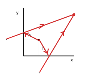
fig. 2. Incorrect Image Theorem source placement for corner cube.


Because of the horizontal orientation of the dipole, I argued that the reflection coefficient should be -1. The reflection point is a bit messy to calculate, and it turns out to zeroth order in \( h/r \) the \( \sin\theta \) magnitude scaling of the reflected (far-field) field is present for both reflected rays. I though that this was probably because the observation point lays at the same altitude for both the line of sight ray and the reflected ray.

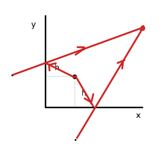
Attempting this problem as a reflection problem makes it much more difficult than it needs to be. It turns out that the correct image source placement for this problem is that of fig. 3.


cornerCubeImageSourcePlacementFig3

fig. 3. Correct image source placement for the corner cube.


This wasn’t at all obvious to me. The key is understanding that the goal of the image source placement isn’t to figure out how the reflection will occur, but to manufacture a source configuration for which the tangential component of the electric field is zero on the conducting surface.

Image placement for infinite conducting plane.

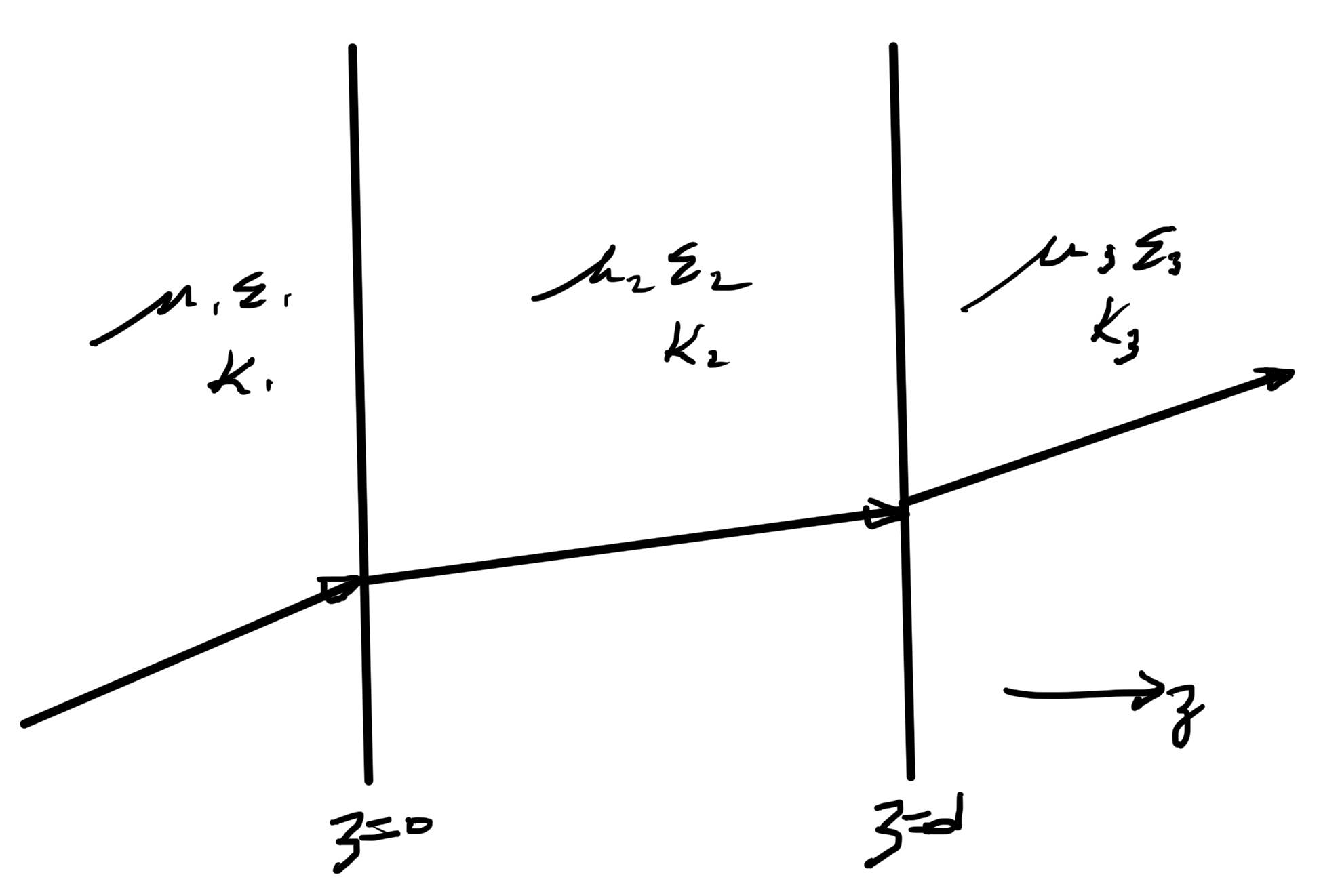
Before thinking about the corner cube configuration, consider a horizontal dipole next to an infinite conducting plane. This, and the correct image source placement is illustrated in fig. 4.


reflectionOfImagePointsFig1

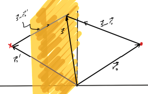
fig. 4. Image source placement for horizontal dipole.


I’ll now verify that this is the correct image source. This is basically a calculation that the tangential components of the electric fields from both sources sum to zero.
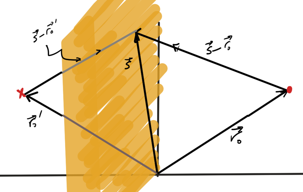
Let,

\begin{equation}\label{eqn:imageTheorem:20}
r = \Abs{\Bs – \Br_0},
\end{equation}

so that the magnetic vector potential for the first quadrant dipole has the form

\begin{equation}\label{eqn:imageTheorem:40}
\BA = \frac{A_0}{4 \pi r} e^{-j k r} \zcap.
\end{equation}

With

\begin{equation}\label{eqn:imageTheorem:60}
\begin{aligned}
\kcap &= \frac{\Bs – \Br_0}{s} \\
\tilde{\BE} &= \zcap – \lr{\zcap \cdot \kcap} \kcap,
\end{aligned}
\end{equation}

the far-field electric field at the point \( \Bs \) on the plane is

\begin{equation}\label{eqn:imageTheorem:80}
\BE = -j \omega \frac{A_0}{4 \pi r} e^{-j k r} \tilde{\BE}.
\end{equation}

If the normal to the plane is \( \ncap \) the tangential component of this field is the projection of \( \BE \) on the direction

\begin{equation}\label{eqn:imageTheorem:100}
\pcap = \frac{\kcap \cross \ncap}{\Abs{\kcap \cross \ncap}}.
\end{equation}

That tangential component is directed along

\begin{equation}\label{eqn:imageTheorem:120}
\lr{\tilde{\BE} \cdot \pcap } \pcap
=
\lr{\lr{\zcap – \lr{\zcap \cdot \kcap} \kcap} \cdot \lr{\kcap \cross \ncap}} \frac{\kcap \cross \ncap}{\Abs{\kcap \cross \ncap}^2}.
\end{equation}

Because the triple product \( \kcap \cdot \lr{\kcap \cross \ncap} = 0 \), the tangential component of the electric field, provided \( \kcap \cdot \ncap \ne 0 \), is

\begin{equation}\label{eqn:imageTheorem:140}
\BE_\parallel
=
-j \omega \frac{A_0}{4 \pi r} e^{-j k r} \zcap \cdot \lr{\kcap \cross \ncap} \frac{\kcap \cross \ncap}{ 1 – \lr{ \ncap \cdot \kcap }^2 }.
\end{equation}

Now the wave vector direction for the second quadrant ray on the plane is required. Both \( \kcap’ \) and \( \Bs’ \) are reflections across the plane. Any such reflection has the value

\begin{equation}\label{eqn:imageTheorem:160}
\begin{aligned}
\Bx’
&= \lr{ \Bx \wedge \ncap} \ncap – \lr{ \Bx \cdot \ncap } \ncap \\
&= – \lr{ \ncap \wedge \Bx + \ncap \cdot \Bx } \ncap \\
&= – \ncap \Bx \ncap.
\end{aligned}
\end{equation}

This multivector product nicely encapsulates the reflection operation. Consider a reflection against the y-z plane with normal \( \Be_1 \) to verify that this works

\begin{equation}\label{eqn:imageTheorem:180}
\begin{aligned}
-\Be_1 \Bx \Be_1
&=
-\Be_1 \lr{ x \Be_1 + y \Be_2 + z \Be_3 } \Be_1 \\
&=
-\lr{ x – y \Be_2 \Be_1 + z \Be_3 \Be_1 } \Be_1 \\
&=
-\lr{ x \Be_1 – y \Be_2 + z \Be_3 } \\
&=
– x \Be_1 + y \Be_2 + z \Be_3.
\end{aligned}
\end{equation}

This has the x component flipped in sign and the rest left untouched as desired for a reflection in the y-z plane.

The second quadrant field will have \( \kcap’ \cross \ncap \) terms in place of all the \( \kcap \cross \ncap \) terms of \ref{eqn:imageTheorem:140}. We want to know how the two compare. This calculation is simply done using the dual form of the cross product temporarily

\begin{equation}\label{eqn:imageTheorem:200}
\begin{aligned}
\kcap’ \cross \ncap
&=
-I \lr{ \kcap’ \wedge \ncap} \\
&=
-I \gpgradetwo{\kcap’ \ncap} \\
&=
-I \gpgradetwo{ {-\ncap \kcap \ncap} \ncap} \\
&=
I \gpgradetwo{ \ncap \kcap } \\
&=
I \ncap \wedge \kcap \\
&=
-\ncap \cross \kcap \\
&=
\kcap \cross \ncap.
\end{aligned}
\end{equation}

So, provided the image source in the second quadrant is oppositely oriented (sign inversion), the tangential components of the two will sum to zero on that surface.

Thinking back to the corner cube, it is clear that an image source opposite to the source across from one of the walls will result in a zero tangential electric field along this boundary as is the case here (say the y-z plane). A second pair of sources opposite from each other anywhere else also about the y-z plane will not change that zero tangential electric field on this surface, but if the signs of the sources is alternated as in fig. 3 it will also result in zero tangential electric field on the z-x plane, which has the desired boundary value effects for both surfaces of the corner cube.