[Click here for a PDF of this post with nicer formatting]
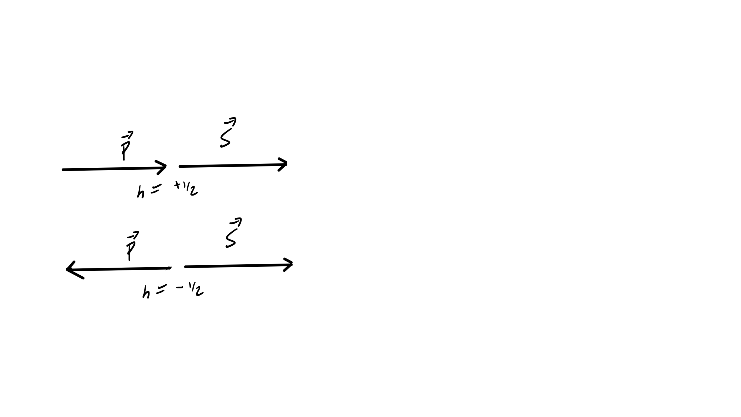
In class yesterday (lecture 19, notes not yet posted) we used \( \Bsigma^\T = -\sigma_2 \Bsigma \sigma_2 \), which implicitly shows that \( (\Bsigma \cdot \Bx)^\T \) is a reflection about the y-axis.
This form of reflection will be familiar to a student of geometric algebra (see [1] — a great book, one copy of which is in the physics library). I can’t recall any mention of the geometrical reflection identity from when I took QM. It’s a fun exercise to demonstrate the reflection identity when constrained to the Pauli matrix notation.
Theorem: Reflection about a normal.
Given a unit vector \( \ncap \in \mathbb{R}^3 \) and a vector \( \Bx \in \mathbb{R}^3 \) the reflection of \( \Bx \) about a plane with normal \( \ncap \) can be represented in Pauli notation as
\begin{equation*}
-\Bsigma \cdot \ncap \Bsigma \cdot \Bx \Bsigma \cdot \ncap.
\end{equation*}
To prove this, first note that in standard vector notation, we can decompose a vector into its projective and rejective components
\begin{equation}\label{eqn:reflection:20}
\Bx = (\Bx \cdot \ncap) \ncap + \lr{ \Bx – (\Bx \cdot \ncap) \ncap }.
\end{equation}
A reflection about the plane normal to \( \ncap \) just flips the component in the direction of \( \ncap \), leaving the rest unchanged. That is
\begin{equation}\label{eqn:reflection:40}
-(\Bx \cdot \ncap) \ncap + \lr{ \Bx – (\Bx \cdot \ncap) \ncap }
=
\Bx – 2 (\Bx \cdot \ncap) \ncap.
\end{equation}
We may write this in \( \Bsigma \) notation as
\begin{equation}\label{eqn:reflection:60}
\Bsigma \cdot \Bx – 2 \Bx \cdot \ncap \Bsigma \cdot \ncap.
\end{equation}
We also know that
\begin{equation}\label{eqn:reflection:80}
\begin{aligned}
\Bsigma \cdot \Ba \Bsigma \cdot \Bb &= a \cdot b + i \Bsigma \cdot (\Ba \cross \Bb) \\
\Bsigma \cdot \Bb \Bsigma \cdot \Ba &= a \cdot b – i \Bsigma \cdot (\Ba \cross \Bb),
\end{aligned}
\end{equation}
or
\begin{equation}\label{eqn:reflection:100}
a \cdot b = \inv{2} \symmetric{\Bsigma \cdot \Ba}{\Bsigma \cdot \Bb},
\end{equation}
where \( \symmetric{\Ba}{\Bb} \) is the anticommutator of \( \Ba, \Bb \).
Inserting \ref{eqn:reflection:100} into \ref{eqn:reflection:60} we find that the reflection is
\begin{equation}\label{eqn:reflection:120}
\begin{aligned}
\Bsigma \cdot \Bx –
\symmetric{\Bsigma \cdot \ncap}{\Bsigma \cdot \Bx}
\Bsigma \cdot \ncap
&=
\Bsigma \cdot \Bx –
{\Bsigma \cdot \ncap}{\Bsigma \cdot \Bx}
\Bsigma \cdot \ncap
–
{\Bsigma \cdot \Bx}{\Bsigma \cdot \ncap}
\Bsigma \cdot \ncap \\
&=
\Bsigma \cdot \Bx –
{\Bsigma \cdot \ncap}{\Bsigma \cdot \Bx}
\Bsigma \cdot \ncap
–
{\Bsigma \cdot \Bx} \\
&=
–
{\Bsigma \cdot \ncap}{\Bsigma \cdot \Bx}
\Bsigma \cdot \ncap,
\end{aligned}
\end{equation}
which completes the proof.
When we expand \( (\Bsigma \cdot \Bx)^\T \) and find
\begin{equation}\label{eqn:reflection:n}
(\Bsigma \cdot \Bx)^\T
=
\sigma^1 x^1 – \sigma^2 x^2 + \sigma^3 x^3,
\end{equation}
it is clear that this coordinate expansion is a reflection about the y-axis. Knowing the reflection formula above provides a rationale for why we might want to write this in the compact form \( -\sigma^2 (\Bsigma \cdot \Bx) \sigma^2 \), which might not be obvious otherwise.
References
[1] C. Doran and A.N. Lasenby. Geometric algebra for physicists. Cambridge University Press New York, Cambridge, UK, 1st edition, 2003.