Month: December 2018

Final first draft of complete notes for UofT PHY2403, QFT I .

December 27, 2018 phy2403 , ,

I’ve now uploaded a new version of my class notes for PHY2403, the UofT Quantum Field Theory I course, taught this year by Prof. Erich Poppitz.

This update adds notes for all remaining lectures (up to and including lecture 23.)  I’ve made a pass with a spellchecker to correct some of the aggregious spelling erorss, and also redrawn three figures, replacing photos, which cuts the size in half!

I’ve posted the redacted version (316 pages).  The full version, with my problem set solutions (including errors) is 409 pages.

Feel free to contact me for the complete version (i.e. including my problem set solutions, with errors) of any of these notes, provided you are not asking because you are taking or planning to take this course.

Contents:

  • Preface
  • Contents
  • List of Figures
  • 1 Fields, units, and scales.
  • 1.1 What is a field?
  • 1.2 Scales.
  • 1.2.1 Bohr radius.
  • 1.2.2 Compton wavelength.
  • 1.2.3 Relations.
  • 1.3 Natural units.
  • 1.4 Gravity.
  • 1.5 Cross section.
  • 1.6 Problems.
  • 2 Lorentz transformations.
  • 2.1 Lorentz transformations.
  • 2.2 Determinant of Lorentz transformations.
  • 2.3 Problems.
  • 3 Classical field theory.
  • 3.1 Field theory.
  • 3.2 Actions.
  • 3.3 Principles determining the form of the action.
  • 3.4 Principles (cont.)
  • 3.4.1 d = 2.
  • 3.4.2 d = 3.
  • 3.4.3 d = 4.
  • 3.4.4 d = 5.
  • 3.5 Least action principle.
  • 3.6 Problems.
  • 4 Canonical quantization, Klein-Gordon equation, SHOs, momentum space representation, raising and lowering operators.
  • 4.1 Canonical quantization.
  • 4.2 Canonical quantization (cont.)
  • 4.3 Momentum space representation.
  • 4.4 Quantization of Field Theory.
  • 4.5 Free Hamiltonian.
  • 4.6 QM SHO review.
  • 4.7 Discussion.
  • 4.8 Problems.
  • 5 Symmetries.
  • 5.1 Switching gears: Symmetries.
  • 5.2 Symmetries.
  • 5.3 Spacetime translation.
  • 5.4 1st Noether theorem.
  • 5.5 Unitary operators.
  • 5.6 Continuous symmetries.
  • 5.7 Classical scalar theory.
  • 5.8 Last time.
  • 5.9 Examples of symmetries.
  • 5.10 Scale invariance.
  • 5.11 Lorentz invariance.
  • 5.12 Problems.
  • 6 Lorentz boosts, generators, Lorentz invariance, microcausality.
  • 6.1 Lorentz transform symmetries.
  • 6.2 Transformation of momentum states.
  • 6.3 Relativistic normalization.
  • 6.4 Spacelike surfaces.
  • 6.5 Condition on microcausality.
  • 7 External sources.
  • 7.1 Harmonic oscillator.
  • 7.2 Field theory (where we are going).
  • 7.3 Green’s functions for the forced Klein-Gordon equation.
  • 7.4 Pole shifting.
  • 7.5 Matrix element representation of the Wightman function.
  • 7.6 Retarded Green’s function.
  • 7.7 Review: “particle creation problem”.
  • 7.8 Digression: coherent states.
  • 7.9 Problems.
  • 8 Perturbation theory.
  • 8.1 Feynman’s Green’s function.
  • 8.2 Interacting field theory: perturbation theory in QFT.
  • 8.3 Perturbation theory, interaction representation and Dyson formula.
  • 8.4 Next time.
  • 8.5 Review.
  • 8.6 Perturbation.
  • 8.7 Review.
  • 8.8 Unpacking it.
  • 8.9 Calculating perturbation.
  • 8.10 Wick contractions.
  • 8.11 Simplest Feynman diagrams.
  • 8.12 Phi fourth interaction.
  • 8.13 Tree level diagrams.
  • 8.14 Problems.
  • 9 Scattering and decay.
  • 9.1 Additional resources.
  • 9.2 Definitions and motivation.
  • 9.3 Calculating interactions.
  • 9.4 Example diagrams.
  • 9.5 The recipe.
  • 9.6 Back to our scalar theory.
  • 9.7 Review: S-matrix.
  • 9.8 Scattering in a scalar theory.
  • 9.9 Decay rates.
  • 9.10 Cross section.
  • 9.11 More on cross section.
  • 9.12 d(LIPS)_2.
  • 9.13 Problems.
  • 10 Fermions, and spinors.
  • 10.1 Fermions: R3 rotations.
  • 10.2 Lorentz group.
  • 10.3 Weyl spinors.
  • 10.4 Lorentz symmetry.
  • 10.5 Dirac matrices.
  • 10.6 Dirac Lagrangian.
  • 10.7 Review.
  • 10.8 Dirac equation.
  • 10.9 Helicity.
  • 10.10 Next time.
  • 10.11 Review.
  • 10.12 Normalization.
  • 10.13 Other solution.
  • 10.14 Lagrangian.
  • 10.15 General solution and Hamiltonian.
  • 10.16 Review.
  • 10.17 Hamiltonian action on single particle states.
  • 10.18 Spacetime translation symmetries.
  • 10.19 Rotation symmetries: angular momentum operator.
  • 10.20 U(1)_V symmetry: charge!
  • 10.21 U(1)_A symmetry: what was the charge for this one called?
  • 10.22 CPT symmetries.
  • 10.23 Review.
  • 10.24 Photon.
  • 10.25 Propagator.
  • 10.26 Feynman rules.
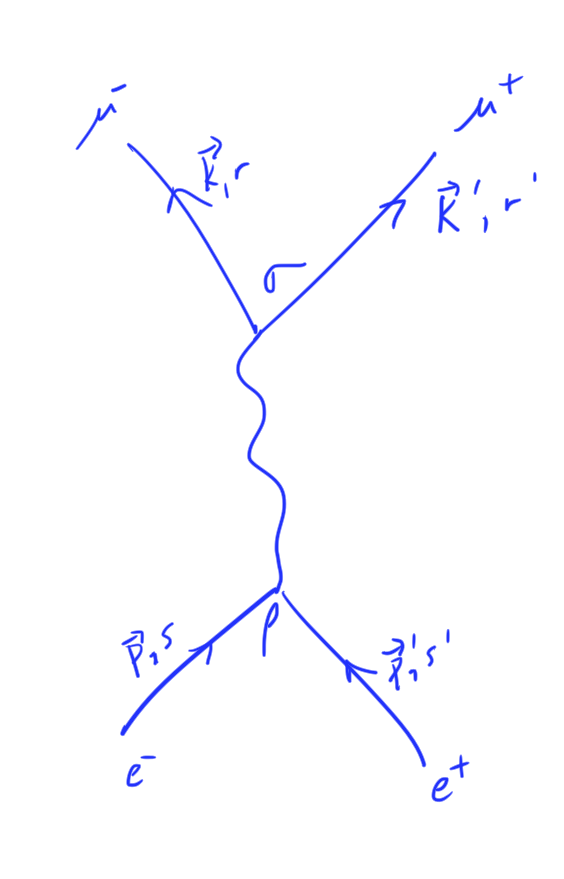
  • 10.27 Example: muon pair production
  • 10.28 Measurement of intermediate quark scattering processes.
  • 10.29 Problems.
  • A Useful formulas and review.
  • A.1 Review of old material.
  • A.2 Useful results from new material.
  • B Momentum of scalar field.
  • B.1 Expansion of the field momentum.
  • B.2 Conservation of the field momentum.
  • C Reflection using Pauli matrices.
  • D Explicit expansion of the Dirac u,v spinors.
  • D.1 Compact representation of
  • E Mathematica notebooks
  • Bibliography

PHY2403H Quantum Field Theory. Lecture 23: QED and QCD interaction Lagrangian, Feynman propagator and rules for Fermions, hadron pair production, scattering cross section, quark pair production. Taught by Prof. Erich Poppitz

December 26, 2018 phy2403 , , , , , , , , , , , , , , , ,

Here is a link to [a PDF with my notes for the final QFT I lecture.] That lecture followed [1] section 5.1 fairly closely (filling in some details, leaving out some others.)

This lecture

  • Introduced an interaction Lagrangian with QED and QCD interaction terms
    \begin{equation*}
    \LL_{\text{QED}}
    =
    – \inv{4} F_{\mu\nu} F^{\mu\nu}
    +
    \overline{\Psi}_e \lr{ i \gamma^\mu \partial_\mu – m } \Psi_e

    e \overline{\Psi}_e \gamma_\mu \Psi_e A^\mu
    +
    \overline{\Psi}_\mu \lr{ i \gamma^\mu \partial_\mu – m } \Psi_\mu

    e \overline{\Psi}_\mu \gamma_\mu \Psi_\mu A^\mu,
    \end{equation*}
    as well as the quark interaction Lagrangian
    \begin{equation*}
    \LL_{\text{quarks}} = \sum_q \overline{\Psi}_q \lr{ i \gamma^\mu – m_q } \Psi_q + e Q_q \overline{\Psi}_q \gamma^\nu \Psi_q A_\nu.
    \end{equation*}
  • The Feynman propagator for Fermions was calculated
    \begin{equation*}
    \expectation{ T( \Psi_\alpha(x) \Psi_\beta(x) }_0
    =
    \lr{ \gamma^\mu_{\alpha\beta} \partial_\mu^{(x)} + m } D_F(x – y)
    =
    \int \frac{d^4 p}{(2 \pi)^4 } \frac{ i ( \gamma^\mu_{\alpha\beta} p_\mu + m ) }{p^2 – m^2 + i \epsilon} e^{-i p \cdot (x – y)}.
    \end{equation*}
  • We determined the Feynman rules for Fermion diagram nodes and edges.
    The Feynman propagator for Fermions is
    \begin{equation*}
    \frac{ i \lr{ \gamma^\mu p_\mu + m } }{p^2 – m^2 + i \epsilon},
    \end{equation*}
    whereas the photon propagator is
    \begin{equation*}
    \expectation{ A_\mu A_\nu } = -i \frac{g_{\mu\nu}}{q^2 + i \epsilon}.
    \end{equation*}
  • Muon pair production

    We then studied muon pair production in detail, and determined the form of the scattering matrix element
    \begin{equation*}
    i M
    =
    i \frac{e^2}{q^2}
    \overline{v}^{s’}(p’) \gamma^\rho u^s(p)
    \overline{u}^r(k) \gamma_\rho v^{r’}(k’),
    \end{equation*}
    where the \( (2 \pi)^4 \delta^4(…) \) term hasn’t been made explicit, and detemined that the average of its square over all input and output polarization (spin) states was
    \begin{equation*}
    \inv{4} \sum_{ss’, rr’} \Abs{M}^2
    =
    \frac{e^4}{4 q^4}
    \textrm{tr}{ \lr{
    \lr{ \gamma^\alpha {k’}_\alpha – m_\mu }
    \gamma_\nu
    \lr{ \gamma^\beta {k}_\beta + m_\mu }
    \gamma_\mu
    }}
    \times
    \textrm{tr}{ \lr{
    \lr{ \gamma^\kappa {p}_\kappa + m_e }
    \gamma^\nu
    \lr{ \gamma^\rho {p’}_\rho – m_e }
    \gamma^\mu
    }}.
    \end{equation*}.
    In the CM frame (neglecting the electron mass, which is small relative to the muon mass), this reduced to
    \begin{equation*}
    \inv{4} \sum_{\text{spins}} \Abs{M}^2
    =
    \frac{8 e^4}{q^4}
    \lr{
    p \cdot k’ p’ \cdot k
    + p \cdot k p’ \cdot k’
    + p \cdot p’ m_\mu^2
    }.
    \end{equation*}

  • We computed the differential cross section
    \begin{equation*}
    {\frac{d\sigma}{d\Omega}}_{\text{CM}}
    =
    \frac{\alpha^2}{4 E_{\text{CM}}^2 }
    \sqrt{ 1 – \frac{m_\mu^2}{E^2} }
    \lr{
    1 + \frac{m_\mu^2}{E^2}
    + \lr{ 1 – \frac{m_\mu^2}{E^2} } \cos^2\theta
    },
    \end{equation*}
    and the total cross section
    \begin{equation*}
    \sigma_{\text{total}}
    =
    \frac{4 \pi \alpha^2}{3 E_{\text{CM}}^2 }
    \sqrt{ 1 – \frac{m_\mu^2}{E^2} }
    \lr{
    1 + \inv{2} \frac{m_\mu^2}{E^2}
    },
    \end{equation*}
    and compared that to the cross section that we was determined with the dimensional analysis handwaving at the start of the course.
  • We finished off with a quick discussion of quark pair production, and how some of the calculations we performed for muon pair production can be used to measure and validate the intermediate quark states that were theorized as carriers of the strong force.

References

[1] Michael E Peskin and Daniel V Schroeder. An introduction to Quantum Field Theory. Westview, 1995.

Dirac spinor relations after rest frame boost

December 18, 2018 phy2403 , , , , ,

[Click here for a PDF of this post with nicer formatting]

In [1], Prof Osmond explicitly boosts a \( u^s(p_0) \) Dirac spinor from the rest frame with rest frame energy \( p_0 \).
After doing so he claims the identification
\begin{equation}\label{eqn:squarerootpsigma:20}
\begin{aligned}
\sqrt{m} e^{-\inv{2} \eta \sigma^3} &= \sqrt{ p \cdot \sigma } \\
\sqrt{m} e^{\inv{2} \eta \sigma^3} &= \sqrt{ p \cdot \overline{\sigma} },
\end{aligned}
\end{equation}
for the components of \( u^s(\Lambda p_0) \).

Let’s verify this by squaring. First
\begin{equation}\label{eqn:squarerootpsigma:40}
e^{\pm \inv{2} \eta \sigma^3 }
=
\cosh\lr{ \inv{2} \eta \sigma^3 }
\pm
\sinh\lr{ \inv{2} \eta \sigma^3 } \sigma^3,
\end{equation}
which squares to (FIXME: link to uvspinor.nb)
\begin{equation}\label{eqn:squarerootpsigma:60}
\lr{ e^{\pm \inv{2} \eta \sigma^3 } }^2
=
\begin{bmatrix}
e^{\pm \eta} & 0 \\
0 & e^{\mp \eta}
\end{bmatrix}.
\end{equation}

Explicitly boosting the rest energy \( p_0 \) gives
\begin{equation}\label{eqn:squarerootpsigma:80}
\begin{bmatrix}
p_0 \\
0
\end{bmatrix}
\rightarrow
\begin{bmatrix}
\cosh\eta & \sinh\eta \\
\sinh\eta & \cosh\eta \\
\end{bmatrix}
\begin{bmatrix}
p_0 \\
0
\end{bmatrix}
=
p_0
\begin{bmatrix}
\cosh\eta \\
\sinh\eta
\end{bmatrix},
\end{equation}
so after the boost
\begin{equation}\label{eqn:squarerootpsigma:100}
\begin{aligned}
p \cdot \sigma
&\rightarrow
p_0 \lr{ \cosh \eta – \sinh \eta \sigma^3 } \\
&= p_0
\begin{bmatrix}
\cosh\eta – \sinh\eta & 0 \\
0 & \cosh\eta + \sinh\eta
\end{bmatrix} \\
&=
p_0
\begin{bmatrix}
e^{-\eta} & 0 \\
0 & e^{\eta}
\end{bmatrix},
\end{aligned}
\end{equation}
where \( p_0 = m \) is still the rest frame energy. However, according to \ref{eqn:squarerootpsigma:60} this is exactly
\begin{equation}\label{eqn:squarerootpsigma:120}
\lr{\sqrt{m} e^{-\inv{2} \eta \sigma^3 }}^2
\end{equation}

Since \( p \cdot \overline{\sigma} \) flips the signs of the spatial momentum, we have shown that
\begin{equation}\label{eqn:squarerootpsigma:140}
\begin{aligned}
\lr{\sqrt{m} e^{-\inv{2} \eta \sigma^3 }}^2 &= p \cdot \sigma \\
\lr{\sqrt{m} e^{\inv{2} \eta \sigma^3 }}^2 &= p \cdot \overline{\sigma},
\end{aligned}
\end{equation}
which isn’t a full proof of the claimed result (i.e. the most general orientation isn’t considered), but at least validates the claim.

References

[1] Dr. Tobias Osborne. Qft lecture 15, dirac equation, boost from stationary frame. Youtube. URL https://youtu.be/J2lV8uNx0LU?list=PLDfPUNusx1EpRs-wku83aqYSKfR5fFmfS&t=4328. [Online; accessed 18-December-2018].

PHY2403H Quantum Field Theory. Lecture 22: Dirac sea, charges, angular momentum, spin, U(1) symmetries, electrons and positrons. Taught by Prof. Erich Poppitz

December 17, 2018 phy2403 , , , , , , , ,

This post is a synopsis of the material from the second last lecture of QFT I. I missed that class, but worked from notes kindly provided by Emily Tyhurst, and Stefan Divic, filling in enough details that it made sense to me.

[Click here for an unabrided PDF of my full notes on this day’s lecture material.]

Topics covered include

  • The Hamiltonian action on single particle states showed that the Hamiltonian was an energy eigenoperator
    \begin{equation}\label{eqn:qftLecture22:140}
    H \ket{\Bp, r}
    =
    \omega_\Bp \ket{\Bp, r}.
    \end{equation}
  • The conserved Noether current and charge for spatial translations, the momentum operator, was found to be
    \begin{equation}\label{eqn:momentumDirac:260}
    \BP =
    \int d^3 x
    \Psi^\dagger (-i \spacegrad) \Psi,
    \end{equation}
    which could be written in creation and anhillation operator form as
    \begin{equation}\label{eqn:momentumDirac:261}
    \BP = \sum_{s = 1}^2
    \int \frac{d^3 q}{(2\pi)^3} \Bp \lr{
    a_\Bp^{s\dagger}
    a_\Bp^{s}
    +
    b_\Bp^{s\dagger}
    b_\Bp^{s}
    }.
    \end{equation}
    Single particle states were found to be the eigenvectors of this operator, with momentum eigenvalues
    \begin{equation}\label{eqn:momentumDirac:262}
    \BP a_\Bq^{s\dagger} \ket{0} = \Bq (a_\Bq^{s\dagger} \ket{0}).
    \end{equation}
  • The conserved Noether current and charge for a rotation was found. That charge is
    \begin{equation}\label{eqn:qftLecture22:920}
    \BJ = \int d^3 x \Psi^\dagger(x) \lr{ \underbrace{\Bx \cross (-i \spacegrad)}_{\text{orbital angular momentum}} + \inv{2} \underbrace{\mathbf{1} \otimes \Bsigma}_{\text{spin angular momentum}} } \Psi,
    \end{equation}
    where
    \begin{equation}\label{eqn:qftLecture22:260}
    \mathbf{1} \otimes \Bsigma =
    \begin{bmatrix}
    \Bsigma & 0 \\
    0 & \Bsigma
    \end{bmatrix},
    \end{equation}
    which has distinct orbital and spin angular momentum components. Unlike NRQM, we see both types of angular momentum as components of a single operator. It is argued in [3] that for a particle at rest the single particle state is an eigenvector of this operator, with eigenvalues \( \pm 1/2 \) — the Fermion spin eigenvalues!
  • We examined two \( U(1) \) global symmetries. The Noether charge for the “vector” \( U(1) \) symmetry is
    \begin{equation}\label{eqn:qftLecture22:380}
    Q
    =
    \int \frac{d^3 q}{(2\pi)^3} \sum_{s = 1}^2
    \lr{
    a_\Bp^{s \dagger} a_\Bp^s

    b_\Bp^{s \dagger}
    b_\Bp^s
    },
    \end{equation}
    This charge operator characterizes the \( a, b \) operators. \( a \) particles have charge \( +1 \), and \( b \) particles have charge \( -1 \), or vice-versa depending on convention. We call \( a \) the operator for the electron, and \( b \) the operator for the positron.
  • CPT (Charge-Parity-TimeReversal) symmetries were also mentioned, but not covered in class. We were pointed to [2], [3], [4] to start studying that topic.

References

[1] C. Doran and A.N. Lasenby. Geometric algebra for physicists. Cambridge University Press New York, Cambridge, UK, 1st edition, 2003.

[2] Dr. Michael Luke. Quantum Field Theory., 2011. URL https://www.physics.utoronto.ca/~luke/PHY2403F/References_files/lecturenotes.pdf. [Online; accessed 05-Dec-2018].

[3] Michael E Peskin and Daniel V Schroeder. An introduction to Quantum Field Theory. Westview, 1995.

[4] Dr. David Tong. Quantum Field Theory. URL http://www.damtp.cam.ac.uk/user/tong/qft.html.

Explicit form of the square root of p . sigma.

December 10, 2018 phy2403 , , , ,

[Click here for a PDF of this post with nicer formatting]

With the help of Mathematica, a fairly compact form was found for the root of \( p \cdot \sigma \)
\begin{equation}\label{eqn:DiracUVmatricesExplicit:121}
\sqrt{ p \cdot \sigma }
=
\inv{
\sqrt{ \omega_\Bp- \Norm{\Bp} } + \sqrt{ \omega_\Bp+ \Norm{\Bp} }
}
\begin{bmatrix}
\omega_\Bp- p^3 + \sqrt{ \omega_\Bp^2 – \Bp^2 } & – p^1 + i p^2 \\
– p^1 – i p^2 & \omega_\Bp+ p^3 + \sqrt{ \omega_\Bp^2 – \Bp^2 }
\end{bmatrix}.
\end{equation}
A bit of examination shows that we can do much better. The leading scalar term can be simplified by squaring it
\begin{equation}\label{eqn:squarerootpsigma:140}
\begin{aligned}
\lr{ \sqrt{ \omega_\Bp- \Norm{\Bp} } + \sqrt{ \omega_\Bp+ \Norm{\Bp} } }^2
&=
\omega_\Bp- \Norm{\Bp} + \omega_\Bp+ \Norm{\Bp} + 2 \sqrt{ \omega_\Bp^2 – \Bp^2 } \\
&=
2 \omega_\Bp + 2 m,
\end{aligned}
\end{equation}
where the on-shell value of the energy \( \omega_\Bp^2 = m^2 + \Bp^2 \) has been inserted. Using that again in the matrix, we have
\begin{equation}\label{eqn:squarerootpsigma:160}
\begin{aligned}
\sqrt{ p \cdot \sigma }
&=
\inv{\sqrt{ 2 \omega_\Bp + 2 m }}
\begin{bmatrix}
\omega_\Bp- p^3 + m & – p^1 + i p^2 \\
– p^1 – i p^2 & \omega_\Bp+ p^3 + m
\end{bmatrix} \\
&=
\inv{\sqrt{ 2 \omega_\Bp + 2 m }}
\lr{
(\omega_\Bp + m) \sigma^0
-p^1 \begin{bmatrix} 0 & 1 \\ 1 & 0 \\ \end{bmatrix}
-p^2 \begin{bmatrix} 0 & -i \\ i & 0 \\ \end{bmatrix}
-p^3 \begin{bmatrix} 1 & 0 \\ 0 & -1 \\ \end{bmatrix}
} \\
&=
\inv{\sqrt{ 2 \omega_\Bp + 2 m }}
\lr{
(\omega_\Bp + m) \sigma^0
-p^1 \sigma^1
-p^2 \sigma^2
-p^3 \sigma^3
} \\
&=
\inv{\sqrt{ 2 \omega_\Bp + 2 m }}
\lr{
(\omega_\Bp + m) \sigma^0 – \Bsigma \cdot \Bp
}.
\end{aligned}
\end{equation}

We’ve now found a nice algebraic form for these matrix roots
\begin{equation}\label{eqn:squarerootpsigma:180}
\boxed{
\begin{aligned}
\sqrt{p \cdot \sigma} &= \inv{\sqrt{ 2 \omega_\Bp + 2 m }} \lr{ m + p \cdot \sigma } \\
\sqrt{p \cdot \overline{\sigma}} &= \inv{\sqrt{ 2 \omega_\Bp + 2 m }} \lr{ m + p \cdot \overline{\sigma}}.
\end{aligned}}
\end{equation}

As a check, let’s square one of these explicitly
\begin{equation}\label{eqn:squarerootpsigma:101}
\begin{aligned}
\lr{ \sqrt{p \cdot \sigma} }^2
&= \inv{2 \omega_\Bp + 2 m }
\lr{ m^2 + (p \cdot \sigma)^2 + 2 m (p \cdot \sigma) } \\
&= \inv{2 \omega_\Bp + 2 m }
\lr{ m^2 + (\omega_\Bp^2 – 2 \omega_\Bp \Bsigma \cdot \Bp + \Bp^2) + 2 m (p \cdot \sigma) } \\
&= \inv{2 \omega_\Bp + 2 m }
\lr{ 2 \omega_\Bp^2 – 2 \omega_\Bp \Bsigma \cdot \Bp + 2 m (\omega_\Bp – \Bsigma \cdot \Bp) } \\
&= \inv{2 \omega_\Bp + 2 m }
\lr{ 2 \omega_\Bp \lr{ \omega_\Bp + m } – (2 \omega_\Bp + 2 m) \Bsigma \cdot \Bp } \\
&=
\omega_\Bp – \Bsigma \cdot \Bp \\
&=
p \cdot \sigma,
\end{aligned}
\end{equation}
which validates the result.