Here is a link to [a PDF with my notes for the final QFT I lecture.] That lecture followed [1] section 5.1 fairly closely (filling in some details, leaving out some others.)

This lecture

• Introduced an interaction Lagrangian with QED and QCD interaction terms
  \begin{equation*}
  \LL_{\text{QED}}
  =
  – \inv{4} F_{\mu\nu} F^{\mu\nu}
  +
  \overline{\Psi}_e \lr{ i \gamma^\mu \partial_\mu – m } \Psi_e
  –
  e \overline{\Psi}_e \gamma_\mu \Psi_e A^\mu
  +
  \overline{\Psi}_\mu \lr{ i \gamma^\mu \partial_\mu – m } \Psi_\mu
  –
  e \overline{\Psi}_\mu \gamma_\mu \Psi_\mu A^\mu,
  \end{equation*}
  as well as the quark interaction Lagrangian
  \begin{equation*}
  \LL_{\text{quarks}} = \sum_q \overline{\Psi}_q \lr{ i \gamma^\mu – m_q } \Psi_q + e Q_q \overline{\Psi}_q \gamma^\nu \Psi_q A_\nu.
  \end{equation*}
• The Feynman propagator for Fermions was calculated
  \begin{equation*}
  \expectation{ T( \Psi_\alpha(x) \Psi_\beta(x) }_0
  =
  \lr{ \gamma^\mu_{\alpha\beta} \partial_\mu^{(x)} + m } D_F(x – y)
  =
  \int \frac{d^4 p}{(2 \pi)^4 } \frac{ i ( \gamma^\mu_{\alpha\beta} p_\mu + m ) }{p^2 – m^2 + i \epsilon} e^{-i p \cdot (x – y)}.
  \end{equation*}
• We determined the Feynman rules for Fermion diagram nodes and edges.
  The Feynman propagator for Fermions is
  \begin{equation*}
  \frac{ i \lr{ \gamma^\mu p_\mu + m } }{p^2 – m^2 + i \epsilon},
  \end{equation*}
  whereas the photon propagator is
  \begin{equation*}
  \expectation{ A_\mu A_\nu } = -i \frac{g_{\mu\nu}}{q^2 + i \epsilon}.
  \end{equation*}
• 

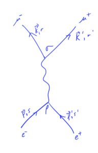
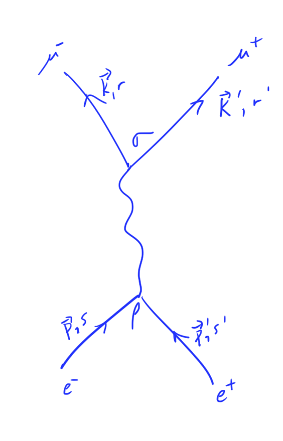
  Muon pair production

  We then studied muon pair production in detail, and determined the form of the scattering matrix element
  \begin{equation*}
  i M
  =
  i \frac{e^2}{q^2}
  \overline{v}^{s’}(p’) \gamma^\rho u^s(p)
  \overline{u}^r(k) \gamma_\rho v^{r’}(k’),
  \end{equation*}
  where the \( (2 \pi)^4 \delta^4(…) \) term hasn’t been made explicit, and detemined that the average of its square over all input and output polarization (spin) states was
  \begin{equation*}
  \inv{4} \sum_{ss’, rr’} \Abs{M}^2
  =
  \frac{e^4}{4 q^4}
  \textrm{tr}{ \lr{
  \lr{ \gamma^\alpha {k’}_\alpha – m_\mu }
  \gamma_\nu
  \lr{ \gamma^\beta {k}_\beta + m_\mu }
  \gamma_\mu
  }}
  \times
  \textrm{tr}{ \lr{
  \lr{ \gamma^\kappa {p}_\kappa + m_e }
  \gamma^\nu
  \lr{ \gamma^\rho {p’}_\rho – m_e }
  \gamma^\mu
  }}.
  \end{equation*}.
  In the CM frame (neglecting the electron mass, which is small relative to the muon mass), this reduced to
  \begin{equation*}
  \inv{4} \sum_{\text{spins}} \Abs{M}^2
  =
  \frac{8 e^4}{q^4}
  \lr{
  p \cdot k’ p’ \cdot k
  + p \cdot k p’ \cdot k’
  + p \cdot p’ m_\mu^2
  }.
  \end{equation*}

• We computed the differential cross section
  \begin{equation*}
  {\frac{d\sigma}{d\Omega}}_{\text{CM}}
  =
  \frac{\alpha^2}{4 E_{\text{CM}}^2 }
  \sqrt{ 1 – \frac{m_\mu^2}{E^2} }
  \lr{
  1 + \frac{m_\mu^2}{E^2}
  + \lr{ 1 – \frac{m_\mu^2}{E^2} } \cos^2\theta
  },
  \end{equation*}
  and the total cross section
  \begin{equation*}
  \sigma_{\text{total}}
  =
  \frac{4 \pi \alpha^2}{3 E_{\text{CM}}^2 }
  \sqrt{ 1 – \frac{m_\mu^2}{E^2} }
  \lr{
  1 + \inv{2} \frac{m_\mu^2}{E^2}
  },
  \end{equation*}
  and compared that to the cross section that we was determined with the dimensional analysis handwaving at the start of the course.
• We finished off with a quick discussion of quark pair production, and how some of the calculations we performed for muon pair production can be used to measure and validate the intermediate quark states that were theorized as carriers of the strong force.

References

[1] Michael E Peskin and Daniel V Schroeder. An introduction to Quantum Field Theory. Westview, 1995.