ece1229

Marks are in for Winter 2016

May 18, 2016 Incoherent ramblings , , , , , , , , , , ,

I started my formal re-education program back in 2010 after 20 years out of school. The first few courses were particularly tough after such a long break from school (and exam based courses still are), but I’m getting the hang of playing that game again. Here’s my score so far:

Crs Code  Title                                    Wgt  Mrk  Grd    CrsAvg
PHY356H1  Quantum Mechanics I                      0.50  78  B+     C+
PHY450H1  Rel Electrodynamics                      0.50  78  B+     *
PHY456H1  Quantum Mechanics II                     0.50  72  B-     C+
PHY454H1  Continuum Mech                           0.50  85  A      B
PHY485H1  Adv Classical Optics                     0.50  85  A      *
PHY452H1  Basic Stat Mechanics                     0.50  81  A-     B-
PHY487H1  Condensed Matter I                       0.50  80  A-     B+
ECE1254H  Modeling of Multiphysics Systems         0.50      A+
ECE1229H  Advanced Antenna Theory                  0.50      A-
PHY1520H  Quantum Mechanics                        0.50      A-
PHY1610H  Scientific Computing for Physicists      0.50      A+     

This last grad course is the only one of which they gave (informally through email) a non-letter grade (97). That one happened to be very well suited to me, and did not have anything based on exams nor on presentations (just assignments). They were demanding assignments (and fun), so I had to work really hard for that 97.

As a returning student I really suck at classes that have marks that are highly biased towards exams. My days of showing up late for class, sleeping through big chunks of the parts that I did get their in time for, and still breezing through the exams are long gone. Somehow in my youth I could do that, and still be able to quickly and easily barf out all the correct exam answers without thinking about it. I got a 99 in first year calculus doing exactly that, although it helped that the Central Technical School’s math department kicked butt, and left Prof Smith with only a review role.

Now I take a lot more time thinking things through, and also take a lot of time writing up my notes (which would sometimes have been spent better doing practise problems). It’s funny thinking back to undergrad where I had such scorn for anybody that took notes. Now I do just that, but in latex. I would be the object of my own scorn X10, if I met my teenage self again!

Tangential and normal field components

May 4, 2015 ece1229 , , , , , , , , , , , , ,

[Click here for a PDF of this post with nicer formatting]

The integral forms of Maxwell’s equations can be used to derive relations for the tangential and normal field components to the sources. These relations were mentioned in class. It’s a little late, but lets go over the derivation. This isn’t all review from first year electromagnetism since we are now using a magnetic source modifications of Maxwell’s equations.

The derivation below follows that of [1] closely, but I am trying it myself to ensure that I understand the assumptions.

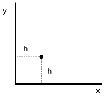
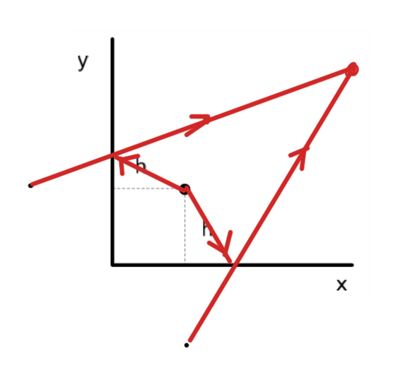
The two infinitesimally thin pillboxes of fig. 1, and fig. 2 are used in the argument.

pillboxForTangentialFieldsFig1

fig. 2: Pillboxes for tangential and normal field relations

pillboxForNormalFieldsFig2

fig. 1: Pillboxes for tangential and normal field relations

Maxwell’s equations with both magnetic and electric sources are

\begin{equation}\label{eqn:normalAndTangentialFields:20}
\spacegrad \cross \boldsymbol{\mathcal{E}} = -\PD{t}{\boldsymbol{\mathcal{B}}} -\boldsymbol{\mathcal{M}}
\end{equation}
\begin{equation}\label{eqn:normalAndTangentialFields:40}
\spacegrad \cross \boldsymbol{\mathcal{H}} = \boldsymbol{\mathcal{J}} + \PD{t}{\boldsymbol{\mathcal{D}}}
\end{equation}
\begin{equation}\label{eqn:normalAndTangentialFields:60}
\spacegrad \cdot \boldsymbol{\mathcal{D}} = \rho_\textrm{e}
\end{equation}
\begin{equation}\label{eqn:normalAndTangentialFields:80}
\spacegrad \cdot \boldsymbol{\mathcal{B}} = \rho_\textrm{m}.
\end{equation}

After application of Stokes’ and the divergence theorems Maxwell’s equations have the integral form

\begin{equation}\label{eqn:normalAndTangentialFields:100}
\oint \boldsymbol{\mathcal{E}} \cdot d\Bl = -\int d\BA \cdot \lr{ \PD{t}{\boldsymbol{\mathcal{B}}} + \boldsymbol{\mathcal{M}} }
\end{equation}
\begin{equation}\label{eqn:normalAndTangentialFields:120}
\oint \boldsymbol{\mathcal{H}} \cdot d\Bl = \int d\BA \cdot \lr{ \PD{t}{\boldsymbol{\mathcal{D}}} + \boldsymbol{\mathcal{J}} }
\end{equation}
\begin{equation}\label{eqn:normalAndTangentialFields:140}
\int_{\partial V} \boldsymbol{\mathcal{D}} \cdot d\BA
=
\int_V \rho_\textrm{e}\,dV
\end{equation}
\begin{equation}\label{eqn:normalAndTangentialFields:160}
\int_{\partial V} \boldsymbol{\mathcal{B}} \cdot d\BA
=
\int_V \rho_\textrm{m}\,dV.
\end{equation}

Maxwell-Faraday equation

First consider one of the loop integrals, like \ref{eqn:normalAndTangentialFields:100}. For an infinestismal loop, that integral is

\begin{equation}\label{eqn:normalAndTangentialFields:180}
\begin{aligned}
\oint \boldsymbol{\mathcal{E}} \cdot d\Bl
&\approx
\mathcal{E}^{(1)}_x \Delta x
+ \mathcal{E}^{(1)} \frac{\Delta y}{2}
+ \mathcal{E}^{(2)} \frac{\Delta y}{2}
-\mathcal{E}^{(2)}_x \Delta x
– \mathcal{E}^{(2)} \frac{\Delta y}{2}
– \mathcal{E}^{(1)} \frac{\Delta y}{2} \\
&\approx
\lr{ \mathcal{E}^{(1)}_x
-\mathcal{E}^{(2)}_x } \Delta x
+ \inv{2} \PD{x}{\mathcal{E}^{(2)}} \Delta x \Delta y
+ \inv{2} \PD{x}{\mathcal{E}^{(1)}} \Delta x \Delta y.
\end{aligned}
\end{equation}

We let \( \Delta y \rightarrow 0 \) which kills off all but the first difference term.

The RHS of \ref{eqn:normalAndTangentialFields:180} is approximately

\begin{equation}\label{eqn:normalAndTangentialFields:200}
-\int d\BA \cdot \lr{ \PD{t}{\boldsymbol{\mathcal{B}}} + \boldsymbol{\mathcal{M}} }
\approx
– \Delta x \Delta y \lr{ \PD{t}{\mathcal{B}_z} + \mathcal{M}_z }.
\end{equation}

If the magnetic field contribution is assumed to be small in comparison to the magnetic current (i.e. infinite magnetic conductance), and if a linear magnetic current source of the form is also assumed

\begin{equation}\label{eqn:normalAndTangentialFields:220}
\boldsymbol{\mathcal{M}}_s = \lim_{\Delta y \rightarrow 0} \lr{\boldsymbol{\mathcal{M}} \cdot \zcap} \zcap \Delta y,
\end{equation}

then the Maxwell-Faraday equation takes the form

\begin{equation}\label{eqn:normalAndTangentialFields:240}
\lr{ \mathcal{E}^{(1)}_x
-\mathcal{E}^{(2)}_x } \Delta x
\approx
– \Delta x \boldsymbol{\mathcal{M}}_s \cdot \zcap.
\end{equation}

While \( \boldsymbol{\mathcal{M}} \) may have components that are not normal to the interface, the surface current need only have a normal component, since only that component contributes to the surface integral.

The coordinate expression of \ref{eqn:normalAndTangentialFields:240} can be written as

\begin{equation}\label{eqn:normalAndTangentialFields:260}
– \boldsymbol{\mathcal{M}}_s \cdot \zcap
=
\lr{ \boldsymbol{\mathcal{E}}^{(1)} -\boldsymbol{\mathcal{E}}^{(2)} } \cdot \lr{ \ycap \cross \zcap }
=
\lr{ \lr{ \boldsymbol{\mathcal{E}}^{(1)} -\boldsymbol{\mathcal{E}}^{(2)} } \cross \ycap } \cdot \zcap.
\end{equation}

This is satisfied when

\begin{equation}\label{eqn:normalAndTangentialFields:280}
\boxed{
\lr{ \boldsymbol{\mathcal{E}}^{(1)} -\boldsymbol{\mathcal{E}}^{(2)} } \cross \ncap = – \boldsymbol{\mathcal{M}}_s,
}
\end{equation}

where \( \ncap \) is the normal between the interfaces. I’d failed to understand when reading this derivation initially, how the \( \boldsymbol{\mathcal{B}} \) contribution was killed off. i.e. If the vanishing area in the surface integral kills off the \( \boldsymbol{\mathcal{B}} \) contribution, why do we have a \( \boldsymbol{\mathcal{M}} \) contribution left. The key to this is understanding that this magnetic current is considered to be confined very closely to the surface getting larger as \( \Delta y \) gets smaller.

Also note that the units of \( \boldsymbol{\mathcal{M}}_s \) are volts/meter like the electric field (not volts/squared-meter like \( \boldsymbol{\mathcal{M}} \).)

Ampere’s law

As above, assume a linear electric surface current density of the form

\begin{equation}\label{eqn:normalAndTangentialFields:300}
\boldsymbol{\mathcal{J}}_s = \lim_{\Delta y \rightarrow 0} \lr{\boldsymbol{\mathcal{J}} \cdot \ncap} \ncap \Delta y,
\end{equation}

in units of amperes/meter (not amperes/meter-squared like \( \boldsymbol{\mathcal{J}} \).)

To apply the arguments above to Ampere’s law, only the sign needs to be adjusted

\begin{equation}\label{eqn:normalAndTangentialFields:290}
\boxed{
\lr{ \boldsymbol{\mathcal{H}}^{(1)} -\boldsymbol{\mathcal{H}}^{(2)} } \cross \ncap = \boldsymbol{\mathcal{J}}_s.
}
\end{equation}

Gauss’s law

Using the cylindrical pillbox surface with radius \( \Delta r \), height \( \Delta y \), and top and bottom surface areas \( \Delta A = \pi \lr{\Delta r}^2 \), the LHS of Gauss’s law \ref{eqn:normalAndTangentialFields:140} expands to

\begin{equation}\label{eqn:normalAndTangentialFields:320}
\begin{aligned}
\int_{\partial V} \boldsymbol{\mathcal{D}} \cdot d\BA
&\approx
\mathcal{D}^{(2)}_y \Delta A
+ \mathcal{D}^{(2)}_\rho 2 \pi \Delta r \frac{\Delta y}{2}
+ \mathcal{D}^{(1)}_\rho 2 \pi \Delta r \frac{\Delta y}{2}
-\mathcal{D}^{(1)}_y \Delta A \\
&\approx
\lr{ \mathcal{D}^{(2)}_y
-\mathcal{D}^{(1)}_y } \Delta A.
\end{aligned}
\end{equation}

As with the Stokes integrals above it is assumed that the height is infinestimal with respect to the radial dimension. Letting that height \( \Delta y \rightarrow 0 \) kills off the radially directed contributions of the flux through the sidewalls.

The RHS expands to approximately

\begin{equation}\label{eqn:normalAndTangentialFields:340}
\int_V \rho_\textrm{e}\,dV
\approx
\Delta A \Delta y \rho_\textrm{e}.
\end{equation}

Define a highly localized surface current density (coulombs/meter-squared) as

\begin{equation}\label{eqn:normalAndTangentialFields:360}
\sigma_\textrm{e} = \lim_{\Delta y \rightarrow 0} \Delta y \rho_\textrm{e}.
\end{equation}

Equating \ref{eqn:normalAndTangentialFields:340} with \ref{eqn:normalAndTangentialFields:320} gives

\begin{equation}\label{eqn:normalAndTangentialFields:380}
\lr{ \mathcal{D}^{(2)}_y
-\mathcal{D}^{(1)}_y } \Delta A
=
\Delta A \sigma_\textrm{e},
\end{equation}

or

\begin{equation}\label{eqn:normalAndTangentialFields:400}
\boxed{
\lr{ \boldsymbol{\mathcal{D}}^{(2)} – \boldsymbol{\mathcal{D}}^{(1)} } \cdot \ncap = \sigma_\textrm{e}.
}
\end{equation}

Gauss’s law for magnetism

The same argument can be applied to the magnetic flux. Define a highly localized magnetic surface current density (webers/meter-squared) as

\begin{equation}\label{eqn:normalAndTangentialFields:440}
\sigma_\textrm{m} = \lim_{\Delta y \rightarrow 0} \Delta y \rho_\textrm{m},
\end{equation}

yielding the boundary relation

\begin{equation}\label{eqn:normalAndTangentialFields:420}
\boxed{
\lr{ \boldsymbol{\mathcal{B}}^{(2)} – \boldsymbol{\mathcal{B}}^{(1)} } \cdot \ncap = \sigma_\textrm{m}.
}
\end{equation}

References

[1] Constantine A Balanis. Advanced engineering electromagnetics, volume 20, chapter Time-varying and time-harmonic electromagnetic fields. Wiley New York, 1989.

Image theorem

March 14, 2015 ece1229 , , , , , , , ,

[Click here for a PDF of this post with nicer formatting]

In the last problem set we examined the array factor for a corner cube configuration, shown in fig. 1.


homework3Fig1

fig. 1. A corner-cube antenna.


Motivation

This is a horizontal dipole antenna placed next to a metallic corner. The radiation at points in the interior of the cube have contributions due to the line of sight field from the antenna as well as reflections. We looked at an approximation of ground reflections using the \underlineAndIndex{Image Theorem}, modeling the ground as a perfectly conducting surface. I completely misunderstood that theorem and how it should be applied. As presented it seemed like a simple way to figure out the reflection characteristics. This confused me since it did not seem consistent with Fresnel reflection theory. I did try to reconcile to the two, but that reconciliation only appeared to work for certain dipole orientations, and that orientation dependence remained an open question.

It turns out that the idea of the Image Theorem is to find a source configuration that contains the specified source, but contains enough other sources that the tangential component of the electric field superposition is zero on the conducting surface, as required by Maxwell’s equations. This allows the boundary to be completely removed from the problem.

Thinking of the corner cube configuration as a reflection problem, I positioned sources as in fig. 2.


incorrectImagePlacementForCornerCubeFig2

fig. 2. Incorrect Image Theorem source placement for corner cube.


Because of the horizontal orientation of the dipole, I argued that the reflection coefficient should be -1. The reflection point is a bit messy to calculate, and it turns out to zeroth order in \( h/r \) the \( \sin\theta \) magnitude scaling of the reflected (far-field) field is present for both reflected rays. I though that this was probably because the observation point lays at the same altitude for both the line of sight ray and the reflected ray.

Attempting this problem as a reflection problem makes it much more difficult than it needs to be. It turns out that the correct image source placement for this problem is that of fig. 3.


cornerCubeImageSourcePlacementFig3

fig. 3. Correct image source placement for the corner cube.


This wasn’t at all obvious to me. The key is understanding that the goal of the image source placement isn’t to figure out how the reflection will occur, but to manufacture a source configuration for which the tangential component of the electric field is zero on the conducting surface.

Image placement for infinite conducting plane.

Before thinking about the corner cube configuration, consider a horizontal dipole next to an infinite conducting plane. This, and the correct image source placement is illustrated in fig. 4.


reflectionOfImagePointsFig1

fig. 4. Image source placement for horizontal dipole.


I’ll now verify that this is the correct image source. This is basically a calculation that the tangential components of the electric fields from both sources sum to zero.

Let,

\begin{equation}\label{eqn:imageTheorem:20}
r = \Abs{\Bs – \Br_0},
\end{equation}

so that the magnetic vector potential for the first quadrant dipole has the form

\begin{equation}\label{eqn:imageTheorem:40}
\BA = \frac{A_0}{4 \pi r} e^{-j k r} \zcap.
\end{equation}

With

\begin{equation}\label{eqn:imageTheorem:60}
\begin{aligned}
\kcap &= \frac{\Bs – \Br_0}{s} \\
\tilde{\BE} &= \zcap – \lr{\zcap \cdot \kcap} \kcap,
\end{aligned}
\end{equation}

the far-field electric field at the point \( \Bs \) on the plane is

\begin{equation}\label{eqn:imageTheorem:80}
\BE = -j \omega \frac{A_0}{4 \pi r} e^{-j k r} \tilde{\BE}.
\end{equation}

If the normal to the plane is \( \ncap \) the tangential component of this field is the projection of \( \BE \) on the direction

\begin{equation}\label{eqn:imageTheorem:100}
\pcap = \frac{\kcap \cross \ncap}{\Abs{\kcap \cross \ncap}}.
\end{equation}

That tangential component is directed along

\begin{equation}\label{eqn:imageTheorem:120}
\lr{\tilde{\BE} \cdot \pcap } \pcap
=
\lr{\lr{\zcap – \lr{\zcap \cdot \kcap} \kcap} \cdot \lr{\kcap \cross \ncap}} \frac{\kcap \cross \ncap}{\Abs{\kcap \cross \ncap}^2}.
\end{equation}

Because the triple product \( \kcap \cdot \lr{\kcap \cross \ncap} = 0 \), the tangential component of the electric field, provided \( \kcap \cdot \ncap \ne 0 \), is

\begin{equation}\label{eqn:imageTheorem:140}
\BE_\parallel
=
-j \omega \frac{A_0}{4 \pi r} e^{-j k r} \zcap \cdot \lr{\kcap \cross \ncap} \frac{\kcap \cross \ncap}{ 1 – \lr{ \ncap \cdot \kcap }^2 }.
\end{equation}

Now the wave vector direction for the second quadrant ray on the plane is required. Both \( \kcap’ \) and \( \Bs’ \) are reflections across the plane. Any such reflection has the value

\begin{equation}\label{eqn:imageTheorem:160}
\begin{aligned}
\Bx’
&= \lr{ \Bx \wedge \ncap} \ncap – \lr{ \Bx \cdot \ncap } \ncap \\
&= – \lr{ \ncap \wedge \Bx + \ncap \cdot \Bx } \ncap \\
&= – \ncap \Bx \ncap.
\end{aligned}
\end{equation}

This multivector product nicely encapsulates the reflection operation. Consider a reflection against the y-z plane with normal \( \Be_1 \) to verify that this works

\begin{equation}\label{eqn:imageTheorem:180}
\begin{aligned}
-\Be_1 \Bx \Be_1
&=
-\Be_1 \lr{ x \Be_1 + y \Be_2 + z \Be_3 } \Be_1 \\
&=
-\lr{ x – y \Be_2 \Be_1 + z \Be_3 \Be_1 } \Be_1 \\
&=
-\lr{ x \Be_1 – y \Be_2 + z \Be_3 } \\
&=
– x \Be_1 + y \Be_2 + z \Be_3.
\end{aligned}
\end{equation}

This has the x component flipped in sign and the rest left untouched as desired for a reflection in the y-z plane.

The second quadrant field will have \( \kcap’ \cross \ncap \) terms in place of all the \( \kcap \cross \ncap \) terms of \ref{eqn:imageTheorem:140}. We want to know how the two compare. This calculation is simply done using the dual form of the cross product temporarily

\begin{equation}\label{eqn:imageTheorem:200}
\begin{aligned}
\kcap’ \cross \ncap
&=
-I \lr{ \kcap’ \wedge \ncap} \\
&=
-I \gpgradetwo{\kcap’ \ncap} \\
&=
-I \gpgradetwo{ {-\ncap \kcap \ncap} \ncap} \\
&=
I \gpgradetwo{ \ncap \kcap } \\
&=
I \ncap \wedge \kcap \\
&=
-\ncap \cross \kcap \\
&=
\kcap \cross \ncap.
\end{aligned}
\end{equation}

So, provided the image source in the second quadrant is oppositely oriented (sign inversion), the tangential components of the two will sum to zero on that surface.

Thinking back to the corner cube, it is clear that an image source opposite to the source across from one of the walls will result in a zero tangential electric field along this boundary as is the case here (say the y-z plane). A second pair of sources opposite from each other anywhere else also about the y-z plane will not change that zero tangential electric field on this surface, but if the signs of the sources is alternated as in fig. 3 it will also result in zero tangential electric field on the z-x plane, which has the desired boundary value effects for both surfaces of the corner cube.

Resolving fields into components parallel to the reflecting plane

March 6, 2015 ece1229 , , , , ,

[Click here for a PDF of this post with nicer formatting]

In order to apply the Fresnel equations, the field components have to be resolved into components where either the electric field or the magnetic field is parallel to the plane of reflection. The geometry of this, with the wave vector direction \( \kcap \) and the electric and magnetic field phasors perpendicular to that direction is sketched in fig. 1.

resolvingFieldsIncidentOnObliquePlaneFig1

fig. 1. Field components relative to reflecting plane


If the incident wave is a plane wave, or equivalently a far field spherical wave, it will have the form

\begin{equation}\label{eqn:resolvingFieldsIncidentOnPlane:20}
\BH = \inv{\mu_0} \kcap \cross \BE,
\end{equation}

with the field directions and wave vector directions satisfying

\begin{equation}\label{eqn:resolvingFieldsIncidentOnPlane:60}
\Ecap \cross \Hcap = \kcap
\end{equation}
\begin{equation}\label{eqn:resolvingFieldsIncidentOnPlane:80}
\Ecap \cdot \kcap = 0
\end{equation}
\begin{equation}\label{eqn:resolvingFieldsIncidentOnPlane:100}
\Hcap \cdot \kcap = 0.
\end{equation}

The key to resolving the fields into components parallel to the plane of reflection lies in the observation that the cross product of the plane normal \( \ncap \) and the incident wave vector direction \( \kcap \) lies in that plane. With

\begin{equation}\label{eqn:resolvingFieldsIncidentOnPlane:140}
\pcap = \frac{\kcap \cross \ncap}{\Abs{\kcap \cross \ncap}}
\end{equation}
\begin{equation}\label{eqn:resolvingFieldsIncidentOnPlane:160}
\qcap = \kcap \cross \pcap,
\end{equation}

the field directions can be resolved into components

\begin{equation}\label{eqn:resolvingFieldsIncidentOnPlane:200}
\BE = \lr{ \BE \cdot \pcap } \pcap + \lr{ \BE \cdot \qcap } \qcap = E_\parallel \pcap + E_\perp \qcap
\end{equation}
\begin{equation}\label{eqn:resolvingFieldsIncidentOnPlane:220}
\BH = \lr{ \BH \cdot \pcap } \pcap + \lr{ \BH \cdot \qcap } \qcap = H_\parallel \pcap + H_\perp \qcap.
\end{equation}

This subdivides the fields into two pairs, one with the electric field parallel to the reflection plane

\begin{equation}\label{eqn:resolvingFieldsIncidentOnPlane:240}
\begin{aligned}
\BE_1 &= \lr{ \BE \cdot \pcap } \pcap = E_\parallel \pcap \\
\BH_1 &= \lr{ \BH \cdot \qcap } \qcap = H_\perp \qcap,
\end{aligned}
\end{equation}

and one with the magnetic field parallel to the reflection plane

\begin{equation}\label{eqn:resolvingFieldsIncidentOnPlane:260}
\begin{aligned}
\BH_2 &= \lr{ \BH \cdot \pcap } \pcap = H_\parallel \pcap \\
\BE_2 &= \lr{ \BE \cdot \qcap } \qcap = E_\perp \qcap.
\end{aligned}
\end{equation}

This is most of what we need to proceed with the reflection and transmission analysis. The only task remaining is to determine the reflection angle.

Using a pencil with the tip on the table I was able to convince myself by observation that there is always a normal plane of incidence regardless of any oblique angle that the ray hits the reflecting surface. This was, for some reason, not intuitively obvious to me. Having done that, the geometry must be reduced to what is sketched in fig. 2.

resolvingAngleOfIncidenceFig1

fig. 2. Angle of incidence determination


Once \( \pcap \) has been determined, regardless of it’s orientation in the reflection plane, the component of \( \kcap \) that is normal, directed towards, the plane of reflection is

\begin{equation}\label{eqn:resolvingFieldsIncidentOnPlane:280}
\kcap – \lr{ \kcap \cdot \pcap } \pcap,
\end{equation}

with (squared) length

\begin{equation}\label{eqn:resolvingFieldsIncidentOnPlane:300}
\begin{aligned}
\lr{ \kcap – \lr{ \kcap \cdot \pcap } \pcap }^2
&=
1 + \lr{ \kcap \cdot \pcap }^2 – 2 \lr{ \kcap \cdot \pcap }^2 \\
&=
1 – \lr{ \kcap \cdot \pcap }^2.
\end{aligned}
\end{equation}

The angle of incidence, relative to the normal to the reflection plane, follows from

\begin{equation}\label{eqn:resolvingFieldsIncidentOnPlane:320}
\begin{aligned}
\cos\theta
&= \kcap \cdot \frac{
\kcap – \lr{ \kcap \cdot \pcap } \pcap }{
\sqrt{
1 – \lr{ \kcap \cdot \pcap }^2
}
} \\
&=
\sqrt{
1 – \lr{ \kcap \cdot \pcap }^2
},
\end{aligned}
\end{equation}

Expanding the dot product above gives

\begin{equation}\label{eqn:resolvingFieldsIncidentOnPlane:360}
\begin{aligned}
\kcap \cdot \pcap’
&=
\kcap \cdot \lr{ \pcap \cross \ncap } \\
&=
\frac{1}{\Abs{\kcap \cross \ncap} } \kcap \cdot \lr{ \lr{\kcap \cross \ncap} \cross \ncap },
\end{aligned}
\end{equation}

where

\begin{equation}\label{eqn:resolvingFieldsIncidentOnPlane:380}
\begin{aligned}
\kcap \cdot \lr{ \lr{\kcap \cross \ncap} \cross \ncap }
&=
k_r \epsilon_{r s t} \lr{\kcap \cross \ncap}_s n_t \\
&=
k_r \epsilon_{r s t} \epsilon_{s a b} k_a n_b n_t \\
&=
-k_r \delta_{r t}^{[a b]} k_a n_b n_t \\
&=
-k_r n_t \lr{ k_r n_t – k_t n_r } \\
&=
-1 + \lr{ \kcap \cdot \ncap}^2.
\end{aligned}
\end{equation}

That gives

\begin{equation}\label{eqn:resolvingFieldsIncidentOnPlane:400}
\begin{aligned}
\kcap \cdot \pcap’
&=
\frac{-1 + \lr{ \kcap \cdot \ncap}^2}{\sqrt{1 – \lr{ \kcap \cdot \ncap}^2} } \\
&=
-\sqrt{1 – \lr{ \kcap \cdot \ncap}^2},
\end{aligned}
\end{equation}

or

\begin{equation}\label{eqn:resolvingFieldsIncidentOnPlane:420}
\begin{aligned}
\cos\theta
&= \sqrt{ 1 – \lr{-\sqrt{1 – \lr{ \kcap \cdot \ncap}^2}}^2 } \\
&= \sqrt{ \lr{ \kcap \cdot \ncap}^2 } \\
&= \kcap \cdot \ncap.
\end{aligned}
\end{equation}

This surprisingly simple result makes so much sense, it is an awful admission of stupidity that I went through all the vector algebra to get it instead of just writing it down directly.

The end result is the reflection angle is given by

\begin{equation}\label{eqn:resolvingFieldsIncidentOnPlane:340}
\boxed{
\theta = \cos^{-1} \kcap \cdot \ncap,
}
\end{equation}

where the reflection plane normal should off the back surface to get the sign right. The only detail left is the vector direction of the reflected ray (as well as the direction for the transmitted ray if that is of interest). The reflected ray direction flips the sign of the normal component of the ray

\begin{equation}\label{eqn:resolvingFieldsIncidentOnPlane:440}
\begin{aligned}
\kcap’
&= -\lr{\kcap \cdot \ncap} \ncap + \lr{ \kcap \wedge \ncap} \ncap \\
&= -\lr{\kcap \cdot \ncap} \ncap + \kcap – \lr{ \ncap \kcap} \cdot \ncap \\
&= \kcap -2 \lr{\kcap \cdot \ncap} \ncap.
\end{aligned}
\end{equation}

Here the sign of the normal doesn’t matter since it only occurs quadratically.

This now supplies everything needed for the application of the Fresnel equations to determine the reflected ray characteristics of an arbitrarily polarized incident field.

Duality transformation of the far field fields.

February 27, 2015 ece1229 , , , ,

We’ve seen that the far field electric and magnetic fields associated with a magnetic vector potential were

\begin{equation}\label{eqn:dualFarField:40}
\BE = -j \omega \textrm{Proj}_\T \BA,
\end{equation}
\begin{equation}\label{eqn:dualFarField:60}
\BH = \inv{\eta} \kcap \cross \BE.
\end{equation}

It’s worth a quick note that the duality transformation for this, referring to [1] tab. 3.2, is

\begin{equation}\label{eqn:dualFarField:100}
\BH = -j \omega \textrm{Proj}_\T \BF
\end{equation}
\begin{equation}\label{eqn:dualFarField:120}
\BE = -\eta \kcap \cross \BH.
\end{equation}

What does \( \BH \) look like in terms of \( \BA \), and \( \BE \) look like in terms of \( \BH \)?

The first is

\begin{equation}\label{eqn:dualFarField:140}
\BH
= -\frac{j \omega}{\eta} \kcap \cross \lr{ \BA – \lr{\BA \cdot \kcap} \kcap },
\end{equation}

in which the \( \kcap \) crossed terms are killed, leaving

\begin{equation}\label{eqn:dualFarField:160}
\BH
= -\frac{j \omega}{\eta} \kcap \cross \BA.
\end{equation}

The electric field follows again using a duality transformation, so in terms of the electric vector potential, is

\begin{equation}\label{eqn:dualFarField:180}
\BE = j \omega \eta \kcap \cross \BF.
\end{equation}

These show explicitly that neither the electric or magnetic far field have any radial component, matching with intuition for transverse propagation of the fields.

References

[1] Constantine A Balanis. Antenna theory: analysis and design. John Wiley & Sons, 3rd edition, 2005.