Yes, I just published an update last week, but here’s another one.
Temporary price drop on hardcover.
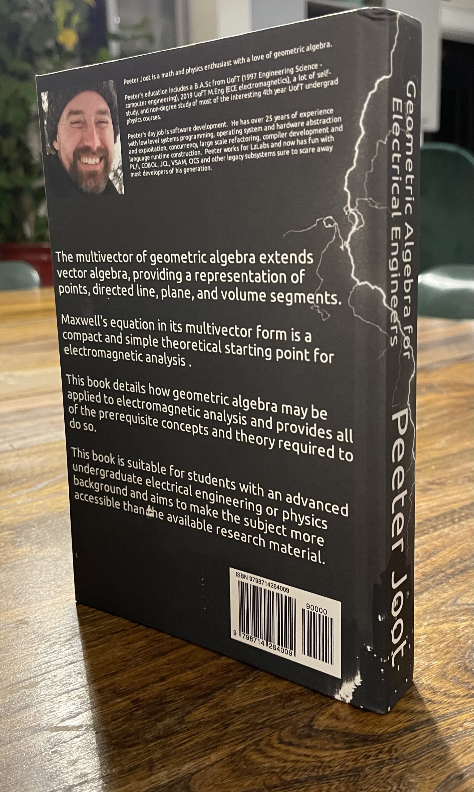
It’s been 4 years since I printed a copy of the book for myself to mark up and edit. In particular, having added some vector calculus identities and their geometric algebra equivalents to chapter II, it messes up the flow a bit, and I’d like a paper copy to review to help figure out how to sequence it all better. I may just start with div and curl (in their GA forms) before moving on to curvilinear coordinates, the vector derivative and all the integration theorems, …
While I intend to mark up my copy, I’m going to treat myself to a hardcover version this time, to see what it looks like.
However, to make things a bit cheaper on myself, I’ve reduced the price on the amazon.com marketplace for the hardcover version of the book to the absolute cheapest amazon will let me make it: $16.12 USD. At that price, amazon will make some profit above printing costs, but I will not. I believe this will also result in a price drop on the amazon.ca marketplace (unlike the paperback pricing, there is no explicit option to set an amazon.ca price for the hardcover version, so I think it’s just the USD price converted to CAD.)
So if you would like a hardcover print copy for yourself at bargain prices, now is your chance. The paperback, in contrast, is $15.50 USD, so for only $0.62 USD more, you (and I) can get a hardcover version! I’ll wait about a week before ordering my copy to make sure that it’s the newest version when I order, and will leave the hardcover price at $16.12 USD until I get my copy in the mail. After that, the price will go back up, and I’ll make a couple bucks for any hardcover sales again after that. Note that the PDF version is still available for free, as always.
If you ask “What about author proofs”. Well, Kindle direct publishing (formerly Createspace) does have a mechanism for ordering author proofs, and if I lived in the USA, I’d use that. However, for us poor second class Canadians, it costs just about as much to get an author proof with shipping, as just buying a copy.
What changed in this version
V0.3.5 (Dec 15, 2023)
- Rewrite spherical polar section with the geometry first, not the coordinate representation, nor the CAS stuff.
- Move the coordinates -> GA derivation to a problem.
- New figure: sphericalPolarFig2.
- update spherical polar figure1 with orientation of j.
- Add to helpful formulas: Vector calculus identities.
- Note about ambiguity of our curl notation.
- Add some references to the d’Alembertian (wave equation) operator.
- New section (chapter 2): Vector calculus identities.
- Two (wedge) curl examples (vector field) to make things less abstract.
- bivector field curl examples (problem.)
- curl with polar form representation of gradient and field (problem.)
- curl of 3D vector field example.