[Click here for a PDF of this post with nicer formatting]

Disclaimer

Peeter’s lecture notes from class. These may be incoherent and rough.

These are notes for the UofT course PHY1520, Graduate Quantum Mechanics, taught by Prof. Paramekanti, covering chap. 4 content from [1].

Parity (review)

\begin{equation}\label{eqn:qmLecture12:20}
\hat{\Pi} \hat{x} \hat{\Pi} = – \hat{x}
\end{equation}
\begin{equation}\label{eqn:qmLecture12:40}
\hat{\Pi} \hat{p} \hat{\Pi} = – \hat{p}
\end{equation}

These are polar vectors, in contrast to an axial vector such as \( \BL = \Br \cross \Bp \).

\begin{equation}\label{eqn:qmLecture12:60}
\hat{\Pi}^2 = 1
\end{equation}

\begin{equation}\label{eqn:qmLecture12:80}
\Psi(x) \rightarrow \Psi(-x)
\end{equation}

If \( \antisymmetric{\hat{\Pi}}{\hat{H}} = 0 \) then all the eigenstates are either

• even: \( \hat{\Pi} \) eigenvalue is \( + 1 \).
• odd: \( \hat{\Pi} \) eigenvalue is \( – 1 \).

We are done with discrete symmetry operators for now.

Translations

Define a (continuous) translation operator

\begin{equation}\label{eqn:qmLecture12:100}
\hat{T}_\epsilon \ket{x} = \ket{x + \epsilon}
\end{equation}

The action of this operator is sketched in fig. 1.

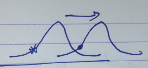
fig. 1. Translation operation.

This is a unitary operator

\begin{equation}\label{eqn:qmLecture12:120}
\hat{T}_{-\epsilon} = \hat{T}_{\epsilon}^\dagger = \hat{T}_{\epsilon}^{-1}
\end{equation}

In a position basis, the action of this operator is

\begin{equation}\label{eqn:qmLecture12:140}
\bra{x} \hat{T}_{\epsilon} \ket{\psi} = \braket{x-\epsilon}{\psi} = \psi(x – \epsilon)
\end{equation}

\begin{equation}\label{eqn:qmLecture12:160}
\Psi(x – \epsilon) \approx \Psi(x) – \epsilon \PD{x}{\Psi}
\end{equation}

\begin{equation}\label{eqn:qmLecture12:180}
\bra{x} \hat{T}_{\epsilon} \ket{\Psi}
= \braket{x}{\Psi} – \frac{\epsilon}{\Hbar} \bra{ x} i \hat{p} \ket{\Psi}
\end{equation}

\begin{equation}\label{eqn:qmLecture12:200}
\hat{T}_{\epsilon} \approx \lr{ 1 – i \frac{\epsilon}{\Hbar} \hat{p} }
\end{equation}

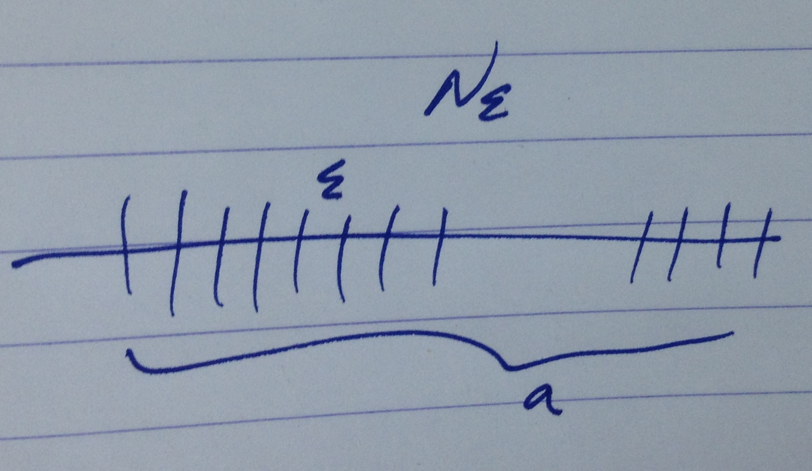
A non-infinitesimal translation can be composed of many small translations, as sketched in fig. 2.

fig. 2. Composition of small translations

For \( \epsilon \rightarrow 0, N \rightarrow \infty, N \epsilon = a \), the total translation operator is

\begin{equation}\label{eqn:qmLecture12:220}
\begin{aligned}
\hat{T}_{a}
&= \hat{T}_{\epsilon}^N \\
&= \lim_{\epsilon \rightarrow 0, N \rightarrow \infty, N \epsilon = a }
\lr{ 1 – \frac{\epsilon}{\Hbar} \hat{p} }^N \\
&= e^{-i a \hat{p}/\Hbar}
\end{aligned}
\end{equation}

The momentum \( \hat{p} \) is called a “Generator” generator of translations. If a Hamiltonian \( H \) is translationally invariant, then

\begin{equation}\label{eqn:qmLecture12:240}
\antisymmetric{\hat{T}_{a}}{H} = 0, \qquad \forall a.
\end{equation}

This means that momentum will be a good quantum number

\begin{equation}\label{eqn:qmLecture12:260}
\antisymmetric{\hat{p}}{H} = 0.
\end{equation}

Rotations

Rotations form a non-Abelian group, since the order of rotations \( \hatR_1 \hatR_2 \ne \hatR_2 \hatR_1 \).

Given a rotation acting on a ket

\begin{equation}\label{eqn:qmLecture12:280}
\hatR \ket{\Br} = \ket{R \Br},
\end{equation}

observe that the action of the rotation operator on a wave function is inverted

\begin{equation}\label{eqn:qmLecture12:300}
\bra{\Br} \hatR \ket{\Psi}
=
\bra{R^{-1} \Br} \ket{\Psi}
= \Psi(R^{-1} \Br).
\end{equation}

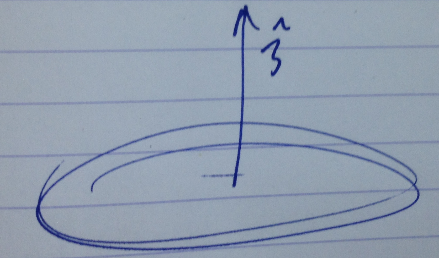
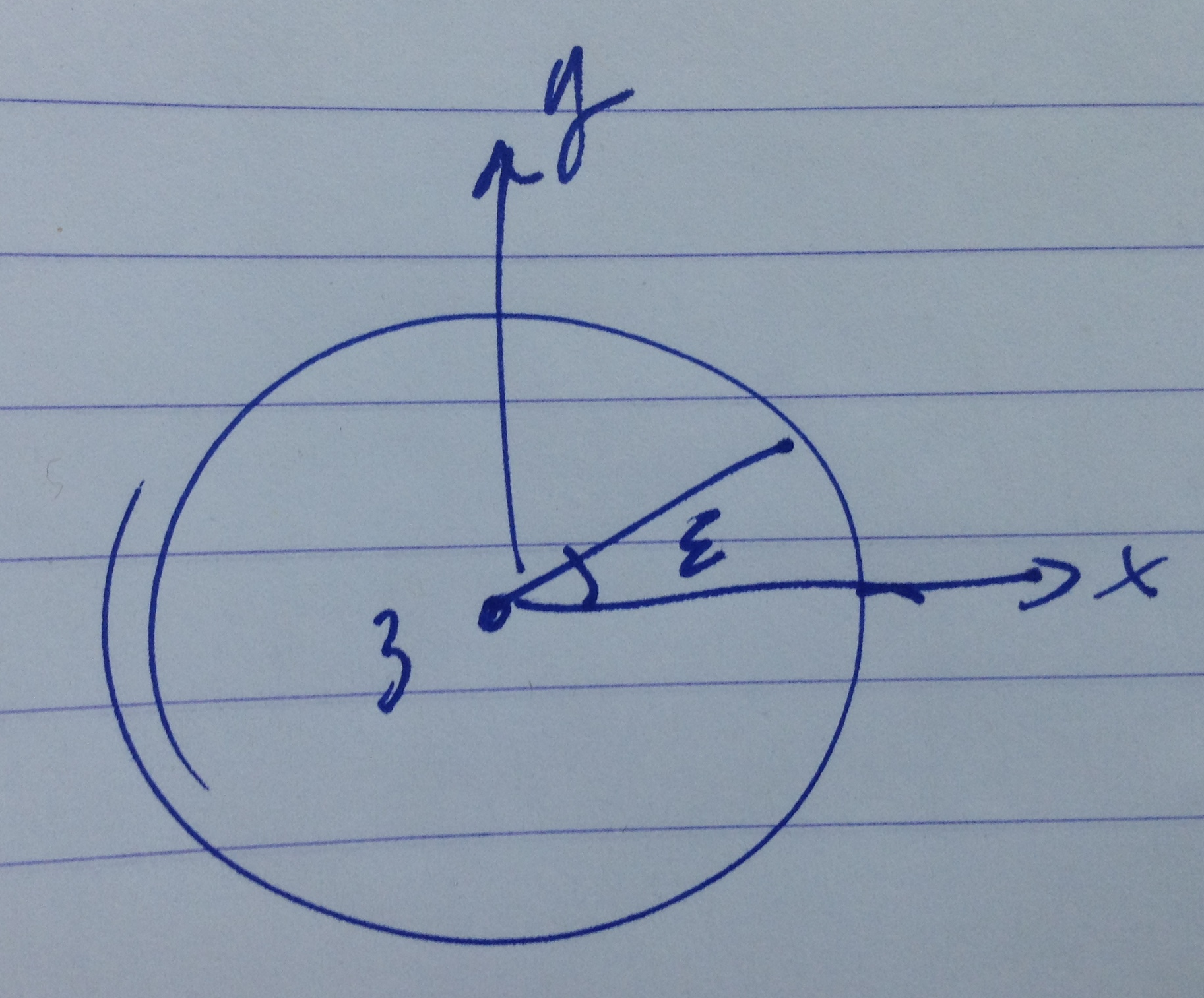
Example: Z axis normal rotation

Consider an infinitesimal rotation about the z-axis as sketched in fig. 3(a),(b)

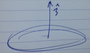
fig 3(a). Rotation about z-axis.

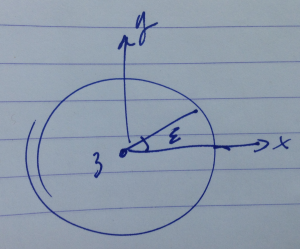
fig 3(b). Rotation about z-axis.

\begin{equation}\label{eqn:qmLecture12:320}
\begin{aligned}
x’ &= x – \epsilon y \\
y’ &= y + \epsilon y \\
z’ &= z
\end{aligned}
\end{equation}

The rotated wave function is

\begin{equation}\label{eqn:qmLecture12:340}
\tilde{\Psi}(x,y,z)
= \Psi( x + \epsilon y, y – \epsilon x, z )
=
\Psi( x, y, z )
+
\epsilon y \underbrace{\PD{x}{\Psi}}_{i \hat{p}_x/\Hbar}
–
\epsilon x \underbrace{\PD{y}{\Psi}}_{i \hat{p}_y/\Hbar}.
\end{equation}

The state must then transform as

\begin{equation}\label{eqn:qmLecture12:360}
\ket{\tilde{\Psi}}
=
\lr{
1
+ i \frac{\epsilon}{\Hbar} \hat{y} \hat{p}_x
– i \frac{\epsilon}{\Hbar} \hat{x} \hat{p}_y
}
\ket{\Psi}.
\end{equation}

Observe that the combination \( \hat{x} \hat{p}_y – \hat{y} \hat{p}_x \) is the \( \hat{L}_z \) component of angular momentum \( \hat{\BL} = \hat{\Br} \cross \hat{\Bp} \), so the infinitesimal rotation can be written

\begin{equation}\label{eqn:qmLecture12:380}
\boxed{
\hatR_z(\epsilon) \ket{\Psi}
=
\lr{ 1 – i \frac{\epsilon}{\Hbar} \hat{L}_z } \ket{\Psi}.
}
\end{equation}

For a finite rotation \( \epsilon \rightarrow 0, N \rightarrow \infty, \phi = \epsilon N \), the total rotation is

\begin{equation}\label{eqn:qmLecture12:420}
\hatR_z(\phi)
=
\lr{ 1 – \frac{i \epsilon}{\Hbar} \hat{L}_z }^N,
\end{equation}

or
\begin{equation}\label{eqn:qmLecture12:440}
\boxed{
\hatR_z(\phi)
=
e^{-i \frac{\phi}{\Hbar} \hat{L}_z}.
}
\end{equation}

Note that \( \antisymmetric{\hat{L}_x}{\hat{L}_y} \ne 0 \).

By construction using Euler angles or any other method, a general rotation will include contributions from components of all the angular momentum operator, and will have the structure

\begin{equation}\label{eqn:qmLecture12:480}
\boxed{
\hatR_\ncap(\phi)
=
e^{-i \frac{\phi}{\Hbar} \lr{ \hat{\BL} \cdot \ncap }}.
}
\end{equation}

Rotationally invariant \( \hat{H} \).

Given a rotationally invariant Hamiltonian

\begin{equation}\label{eqn:qmLecture12:520}
\antisymmetric{\hat{R}_\ncap(\phi)}{\hat{H}} = 0 \qquad \forall \ncap, \phi,
\end{equation}

then every

\begin{equation}\label{eqn:qmLecture12:540}
\antisymmetric{\BL \cdot \ncap}{\hat{H}} = 0,
\end{equation}

or
\begin{equation}\label{eqn:qmLecture12:560}
\antisymmetric{L_i}{\hat{H}} = 0,
\end{equation}

Non-Abelian implies degeneracies in the spectrum.

Time-reversal

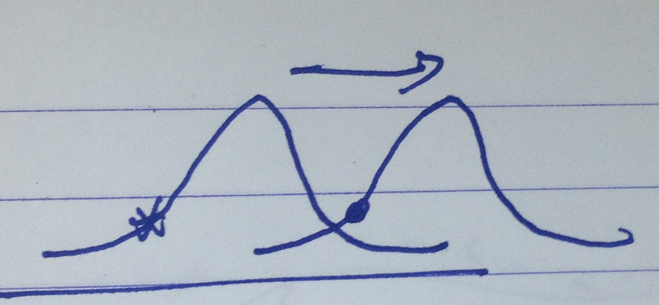
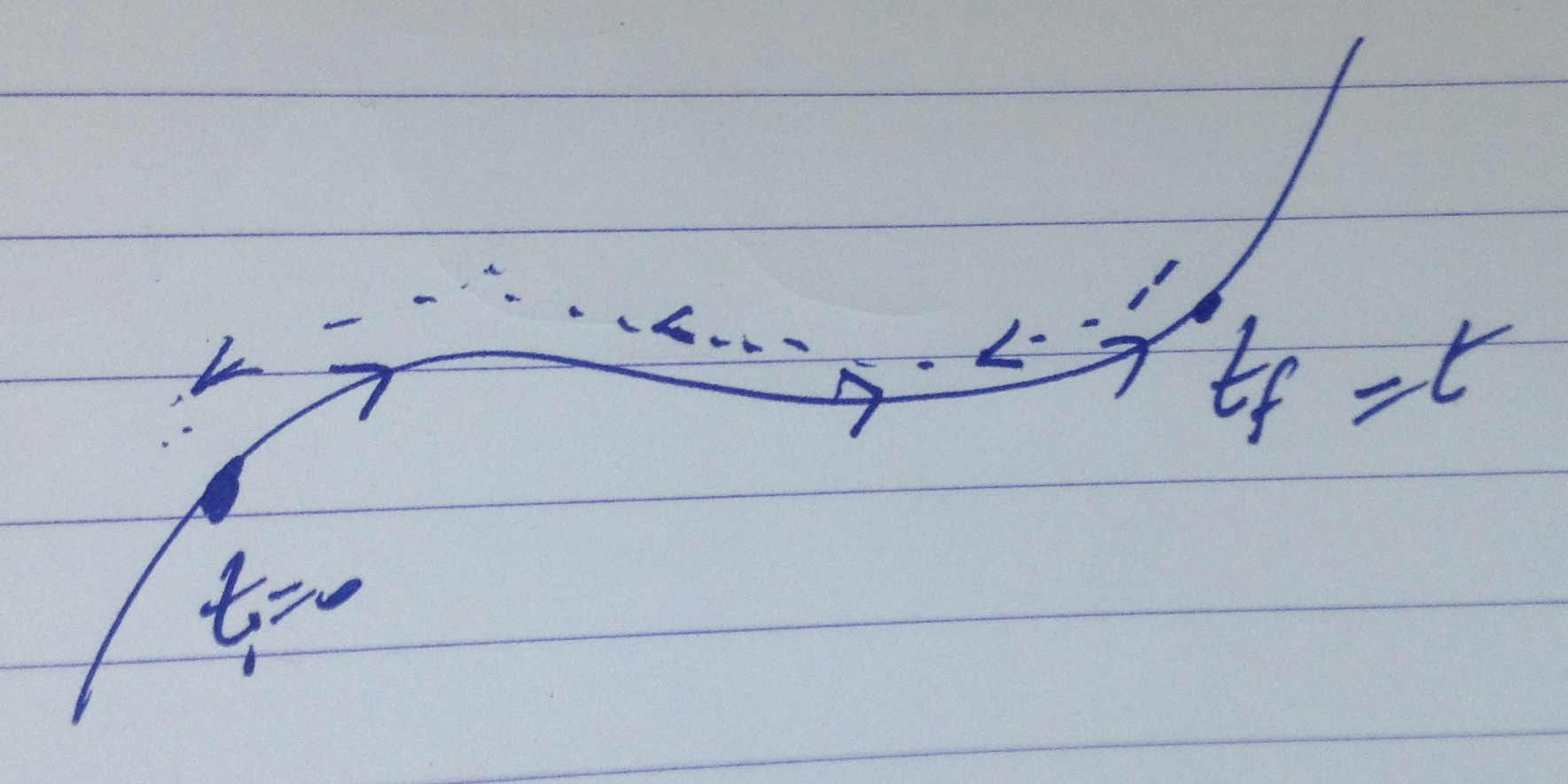
Imagine that we have something moving along a curve at time \( t = 0 \), and ending up at the final position at time \( t = t_f \).

fig. 4. Time reversal trajectory.

Imagine that we flip the direction of motion (i.e. flipping the velocity) and run time backwards so the final-time state becomes the initial state.

If the time reversal operator is designated \( \hat{\Theta} \), with operation

\begin{equation}\label{eqn:qmLecture12:580}
\hat{\Theta} \ket{\Psi} = \ket{\tilde{\Psi}},
\end{equation}

so that

\begin{equation}\label{eqn:qmLecture12:600}
\hat{\Theta}^{-1} e^{-i \hat{H} t/\Hbar} \hat{\Theta} \ket{\Psi(t)} = \ket{\Psi(0)},
\end{equation}

or

\begin{equation}\label{eqn:qmLecture12:620}
\hat{\Theta}^{-1} e^{-i \hat{H} t/\Hbar} \hat{\Theta} \ket{\Psi(0)} = \ket{\Psi(-t)}.
\end{equation}

References

[1] Jun John Sakurai and Jim J Napolitano. Modern quantum mechanics. Pearson Higher Ed, 2014.