Dirac Lagrangian

PHY2403H Quantum Field Theory. Lecture 22: Dirac sea, charges, angular momentum, spin, U(1) symmetries, electrons and positrons. Taught by Prof. Erich Poppitz

December 17, 2018 phy2403 , , , , , , , ,

This post is a synopsis of the material from the second last lecture of QFT I. I missed that class, but worked from notes kindly provided by Emily Tyhurst, and Stefan Divic, filling in enough details that it made sense to me.

[Click here for an unabrided PDF of my full notes on this day’s lecture material.]

Topics covered include

  • The Hamiltonian action on single particle states showed that the Hamiltonian was an energy eigenoperator
    \begin{equation}\label{eqn:qftLecture22:140}
    H \ket{\Bp, r}
    =
    \omega_\Bp \ket{\Bp, r}.
    \end{equation}
  • The conserved Noether current and charge for spatial translations, the momentum operator, was found to be
    \begin{equation}\label{eqn:momentumDirac:260}
    \BP =
    \int d^3 x
    \Psi^\dagger (-i \spacegrad) \Psi,
    \end{equation}
    which could be written in creation and anhillation operator form as
    \begin{equation}\label{eqn:momentumDirac:261}
    \BP = \sum_{s = 1}^2
    \int \frac{d^3 q}{(2\pi)^3} \Bp \lr{
    a_\Bp^{s\dagger}
    a_\Bp^{s}
    +
    b_\Bp^{s\dagger}
    b_\Bp^{s}
    }.
    \end{equation}
    Single particle states were found to be the eigenvectors of this operator, with momentum eigenvalues
    \begin{equation}\label{eqn:momentumDirac:262}
    \BP a_\Bq^{s\dagger} \ket{0} = \Bq (a_\Bq^{s\dagger} \ket{0}).
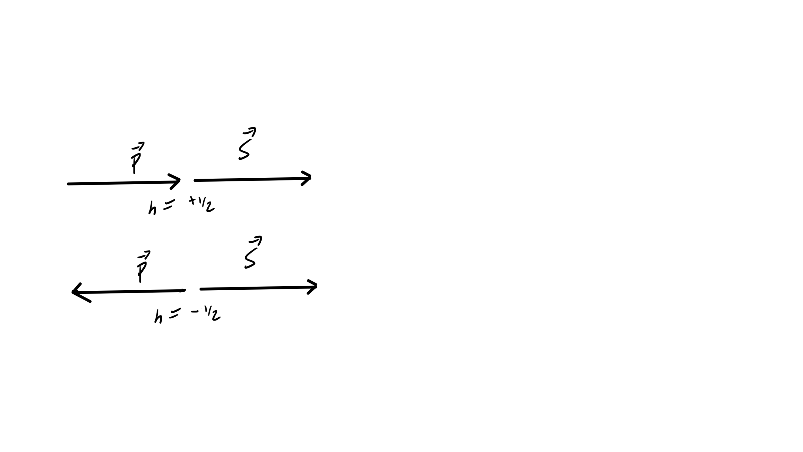
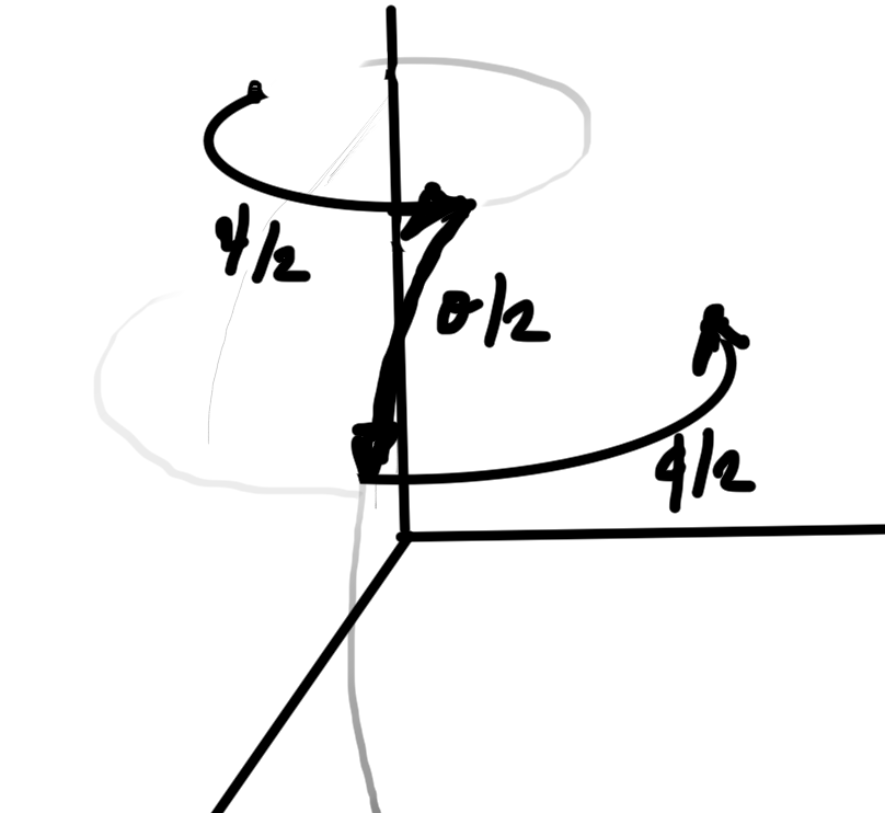
    \end{equation}
  • The conserved Noether current and charge for a rotation was found. That charge is
    \begin{equation}\label{eqn:qftLecture22:920}
    \BJ = \int d^3 x \Psi^\dagger(x) \lr{ \underbrace{\Bx \cross (-i \spacegrad)}_{\text{orbital angular momentum}} + \inv{2} \underbrace{\mathbf{1} \otimes \Bsigma}_{\text{spin angular momentum}} } \Psi,
    \end{equation}
    where
    \begin{equation}\label{eqn:qftLecture22:260}
    \mathbf{1} \otimes \Bsigma =
    \begin{bmatrix}
    \Bsigma & 0 \\
    0 & \Bsigma
    \end{bmatrix},
    \end{equation}
    which has distinct orbital and spin angular momentum components. Unlike NRQM, we see both types of angular momentum as components of a single operator. It is argued in [3] that for a particle at rest the single particle state is an eigenvector of this operator, with eigenvalues \( \pm 1/2 \) — the Fermion spin eigenvalues!
  • We examined two \( U(1) \) global symmetries. The Noether charge for the “vector” \( U(1) \) symmetry is
    \begin{equation}\label{eqn:qftLecture22:380}
    Q
    =
    \int \frac{d^3 q}{(2\pi)^3} \sum_{s = 1}^2
    \lr{
    a_\Bp^{s \dagger} a_\Bp^s

    b_\Bp^{s \dagger}
    b_\Bp^s
    },
    \end{equation}
    This charge operator characterizes the \( a, b \) operators. \( a \) particles have charge \( +1 \), and \( b \) particles have charge \( -1 \), or vice-versa depending on convention. We call \( a \) the operator for the electron, and \( b \) the operator for the positron.
  • CPT (Charge-Parity-TimeReversal) symmetries were also mentioned, but not covered in class. We were pointed to [2], [3], [4] to start studying that topic.

References

[1] C. Doran and A.N. Lasenby. Geometric algebra for physicists. Cambridge University Press New York, Cambridge, UK, 1st edition, 2003.

[2] Dr. Michael Luke. Quantum Field Theory., 2011. URL https://www.physics.utoronto.ca/~luke/PHY2403F/References_files/lecturenotes.pdf. [Online; accessed 05-Dec-2018].

[3] Michael E Peskin and Daniel V Schroeder. An introduction to Quantum Field Theory. Westview, 1995.

[4] Dr. David Tong. Quantum Field Theory. URL http://www.damtp.cam.ac.uk/user/tong/qft.html.

Momentum operator for the Dirac field?

December 8, 2018 phy2403 , , , , ,

[Click here for a PDF of this post with nicer formatting]

In the borrowed notes I have for last Monday’s lecture (which I missed) I see the momentum operator defined by
\begin{equation}\label{eqn:momentumDirac:20}
\BP = \sum_{s = 1}^2
\int \frac{d^3 q}{(2\pi)^3} \Bp \lr{
a_\Bp^{s\dagger}
a_\Bp^{s}
+
b_\Bp^{s\dagger}
b_\Bp^{s}
}.
\end{equation}

There’s a “use Noether’s theorem” comment associated with this. For the scalar field, using Noether’s theorem, we identified the conserved charge of a spacetime translation as the momentum operator
\begin{equation}\label{eqn:momentumDirac:40}
P^i = \int d^3 x T^{0i} = – \int d^3 x \pi(x) \spacegrad \phi(x),
\end{equation}
and if we plugged in the creation and anhillation operator representation of \( \pi, \phi \), out comes
\begin{equation}\label{eqn:momentumDirac:60}
\BP =
\inv{2} \int \frac{d^3 q}{(2\pi)^3} \Bp \lr{ a_\Bp^\dagger a_\Bp + a_\Bp a_\Bp^\dagger},
\end{equation}
(plus \( e^{\pm 2 i \omega_\Bp t} \) terms that we can argue away.)

It wasn’t clear to me how this worked with the Dirac field, but it turns out that this does follow systematically as expected. For a spacetime translation
\begin{equation}\label{eqn:momentumDirac:80}
x^\mu \rightarrow x^\mu + a^\mu,
\end{equation}
we find
\begin{equation}\label{eqn:momentumDirac:100}
\delta \Psi = -a^\mu \partial_\mu \Psi,
\end{equation}
so for the Dirac Lagrangian, we have
\begin{equation}\label{eqn:momentumDirac:120}
\begin{aligned}
\delta \LL
&= \delta \lr{ \overline{\Psi} \lr{ i \gamma^\mu \partial_\mu – m } \Psi } \\
&=
(\delta \overline{\Psi}) \lr{ i \gamma^\mu \partial_\mu – m } \Psi
+
\overline{\Psi} \lr{ i \gamma^\mu \partial_\mu – m } \delta \Psi \\
&=
(-a^\sigma \partial_\sigma \overline{\Psi}) \lr{ i \gamma^\mu \partial_\mu – m } \Psi
+
\overline{\Psi} \lr{ i \gamma^\mu \partial_\mu – m } (-a^\sigma \partial_\sigma \Psi ) \\
&=
-a^\sigma \partial_\sigma \LL \\
&=
\partial_\sigma (-a^\sigma \LL),
\end{aligned}
\end{equation}
i.e. \( J^\mu = -a^\mu \LL \).
To plugging this into the Noether current calculating machine, we have
\begin{equation}\label{eqn:momentumDirac:160}
\begin{aligned}
\PD{(\partial_\mu \Psi)}{\LL}
&=
\PD{(\partial_\mu \Psi)}{} \lr{ \overline{\Psi} i \gamma^\sigma \partial_\sigma \Psi – m \overline{\Psi} \Psi } \\
&=
\overline{\Psi} i \gamma^\mu,
\end{aligned}
\end{equation}
and
\begin{equation}\label{eqn:momentumDirac:180}
\PD{(\partial_\mu \overline{\Psi})}{\LL} = 0,
\end{equation}
so
\begin{equation}\label{eqn:momentumDirac:140}
\begin{aligned}
j^\mu
&=
(\delta \overline{\Psi}) \PD{(\partial_\mu \overline{\Psi})}{\LL}
+
\PD{(\partial_\mu \Psi)}{\LL} (\delta \Psi)
– a^\mu \LL \\
&=
\overline{\Psi} i \gamma^\mu (-a^\sigma \partial_\sigma \Psi)
– a^\sigma {\delta^{\mu}}_{\sigma} \LL \\
&=
– a^\sigma
\lr{
\overline{\Psi} i \gamma^\mu \partial_\sigma \Psi
+ {\delta^{\mu}}_{\sigma} \LL
} \\
&=
-a_\nu
\lr{
\overline{\Psi} i \gamma^\mu \partial^\nu \Psi
+ g^{\mu\nu} \LL
}.
\end{aligned}
\end{equation}

We can now define an energy-momentum tensor
\begin{equation}\label{eqn:momentumDirac:200}
T^{\mu\nu}
=
\overline{\Psi} i \gamma^\mu \partial^\nu \Psi
+ g^{\mu\nu} \LL.
\end{equation}
A couple things are of notable in this tensor. One is that it is not symmetric, and there’s doesn’t appear to be any hope
of making it so. For example, the space+time components are way different
\begin{equation}\label{eqn:momentumDirac:220}
\begin{aligned}
T^{0k} &= \overline{\Psi} i \gamma^0 \partial^k \Psi \\
T^{k0} &= \overline{\Psi} i \gamma^k \partial^0 \Psi,
\end{aligned}
\end{equation}
so if we want a momentum like creature, we have to use \( T^{0k} \), not \( T^{k0} \). The charge associated with that current is
\begin{equation}\label{eqn:momentumDirac:240}
\begin{aligned}
Q^k
&=
\int d^3 x
\overline{\Psi} i \gamma^0 \partial^k \Psi \\
&=
\int d^3 x
\Psi^\dagger (-i \partial_k) \Psi,
\end{aligned}
\end{equation}
or translating from component to vector form
\begin{equation}\label{eqn:momentumDirac:260}
\BP =
\int d^3 x
\Psi^\dagger (-i \spacegrad) \Psi,
\end{equation}
which is the how the momentum operator is first stated in [2]. Here the vector notation doesn’t have any specific representation, but it is interesting to observe how this is directly related to the massless Dirac Lagrangian

\begin{equation}\label{eqn:momentumDirac:280}
\begin{aligned}
\LL(m = 0)
&=
\overline{\Psi} i \gamma^\mu \partial_\mu \Psi \\
&=
\Psi^\dagger i \gamma^\mu \partial_\mu \Psi \\
&=
\Psi^\dagger i (\partial_0 + \gamma_0 \gamma^k \partial_k) \Psi \\
&=
\Psi^\dagger i (\partial_0 – \gamma_0 \gamma_k \partial_k ) \Psi,
\end{aligned}
\end{equation}
but since \( \gamma_0 \gamma_k \) is a \( 4 \times 4 \) representation of the Pauli matrix \( \sigma_k \) Lagrangian itself breaks down into
\begin{equation}\label{eqn:momentumDirac:300}
\LL(m = 0)
=
\Psi^\dagger i \partial_0 \Psi
+
\Bsigma \cdot \lr{ \Psi^\dagger (-i\spacegrad) \Psi },
\end{equation}
components, and lo and behold, out pops the momentum operator density! There is ambiguity as to what order of products \( \gamma_0 \gamma_k \), or \( \gamma_k \gamma_0 \) to pick to represent the Pauli basis ([1] uses \( \gamma_k \gamma_0 \)), but we also have sign ambiguity in assembling a Noether charge from the conserved current, so I don’t think that matters. Some part of this should be expected this since the Dirac equation in momentum space is just \( \gamma \cdot p – m = 0 \), so there is an intimate connection with the operator portion and momentum.

The last detail to fill in is going from \ref{eqn:momentumDirac:260} to \ref{eqn:momentumDirac:20} using the \( a, b\) representation of the field. That’s an algebraically messy looking job that I don’t feel like trying at the moment.

References

[1] C. Doran and A.N. Lasenby. Geometric algebra for physicists. Cambridge University Press New York, Cambridge, UK, 1st edition, 2003.

[2] Michael E Peskin and Daniel V Schroeder. An introduction to Quantum Field Theory. Westview, 1995.

PHY2403H Quantum Field Theory. Lecture 20: Dirac Lagrangian, spinor solutions to the KG equation, Dirac matrices, plane wave solution, helicity. Taught by Prof. Erich Poppitz

November 27, 2018 phy2403 , , , , , , , , ,

[Here is another PDF only post, containing my notes for Lecture 20 of the UofT QFT I (quantum field theory) course.]

In this lecture Professor Poppitz derived a rest frame solution of the Dirac equation, then demonstrated that the generalization to non-zero momentum satisfied the equation. We also saw that Dirac spinor solutions of the Dirac equation are KG equation solutions, and touched on the relation of some solutions to the helicity operator.

This post doesn’t have a web version, since my latex -> wordpress-mathjax script doesn’t have support for the theorem/lemma environments that I used for Monday’s notes, and I don’t have time to implement that right now.

PHY2403H Quantum Field Theory. Lecture 19: Pauli matrices, Weyl spinors, SL(2,c), Weyl action, Weyl equation, Dirac matrix, Dirac action, Dirac Lagrangian. Taught by Prof. Erich Poppitz

November 24, 2018 phy2403 , , , , , , ,

[Here are my notes for lecture 19 of the UofT course PHY2403H, Quantum Field Theory, taught by Prof. Erich Poppitz, fall 2018.] For this lecture my notes are pdf only, due to length. While the after-class length was 8 pages, it ended up expanded to 17 pages by the time I finished making sense of the material.

These also include a portion of the notes from Lecture 18 (not yet posted), as it made sense to group all the Pauli matrix related content.  This particular set of notes diverges from the format presented in class, as it made sense to me to group things in this particular lecture in a more structured definition, theorem, proof style.  I’ve added a number of additional details that I found helpful, as well as a couple of extra problems (some set as formal problems at the end, and others set as theorem or lemmas in with the rest.)