LU factorization

Illustrating the LU algorithm with pivots by example

October 15, 2014 ece1254 , , , ,

[Click here for a PDF of this post with nicer formatting]

Two previous examples of LU factorizations were given. I found one more to be the key to understanding how to implement this as a matlab algorithm, required for our problem set.

A matrix that contains both pivots and elementary matrix operations is

\begin{equation}\label{eqn:luAlgorithm:20}
M=
\begin{bmatrix}
0 & 0 & 2 & 1 \\
0 & 0 & 1 & 1 \\
2 & 0 & 2 & 0 \\
1 & 1 & 1 & 1
\end{bmatrix}
\end{equation}

Our objective is to apply a sequence of row permutations or elementary row operations to \( M \) that put \( M \) into upper triangular form. At the same time we wish to track the all the inverse operations. When no permutations were required to produce \( U \), then we end up with a factorization \( M = L’ U \) where \( L’ \) is lower triangular.

Let’s express the row operations that we apply to \( M \) as

\begin{equation}\label{eqn:luAlgorithm:40}
U =
L_k^{-1}
L_{k-1}^{-1} \cdots
L_2^{-1}
L_1^{-1}
M,
\end{equation}

with

\begin{equation}\label{eqn:luAlgorithm:60}
L’ = L_0 L_1 L_2 \cdots L_{k-1} L_k
\end{equation}

Here \( L_0 = I \), the identity matrix, and \( L_i^{-1} \) is either a permutation matrix interchanging two rows of the identity matrix, or it is an elementary row operation encoding the operation \( r_j \rightarrow r_j – M r_i \), where \( r_i \) is the pivot row, and \( r_j, j > i \) are the rows that we are applying the Gaussian elimination operations to.

For our example matrix, we see that we cannot use the \( M_{1 1} \) as the pivot element since it is zero. In general, for numeric stability, we wish to use the row with the biggest absolute value in the column that we are operating on. In this case that is row 3. Our first row operation is therefore a \( 1,3 \) permutation

\begin{equation}\label{eqn:luAlgorithm:80}
L_1^{-1} =
\begin{bmatrix}
0 & 0 & 1 & 0 \\
0 & 1 & 0 & 0 \\
1 & 0 & 0 & 0 \\
0 & 0 & 0 & 1 \\
\end{bmatrix},
\end{equation}

which gives us

\begin{equation}\label{eqn:luAlgorithm:100}
M \rightarrow
L_1^{-1}
M
=
\begin{bmatrix}
0 & 0 & 1 & 0 \\
0 & 1 & 0 & 0 \\
1 & 0 & 0 & 0 \\
0 & 0 & 0 & 1 \\
\end{bmatrix}
\begin{bmatrix}
0 & 0 & 2 & 1 \\
0 & 0 & 1 & 1 \\
2 & 0 & 2 & 0 \\
1 & 1 & 1 & 1 \\
\end{bmatrix}
=
\begin{bmatrix}
2 & 0 & 2 & 0 \\
0 & 0 & 1 & 1 \\
0 & 0 & 2 & 1 \\
1 & 1 & 1 & 1 \\
\end{bmatrix}.
\end{equation}

Computationally, we do not wish to actually do a matrix multiplication to achieve this permutation. Instead we want to just swap the two rows in question.

The inverse of this operation is the same permutation, so for \( L’ \) we compute

\begin{equation}\label{eqn:luAlgorithm:120}
L’ \rightarrow L_0 L_1 = L_1.
\end{equation}

As before, we don’t wish to do a matrix operation. Since we have applied the permutation matrix from the right, it results in an exchange of columns \(1,3\) of our \( L_0 \) matrix (which happens to be identity at this point). We can implement that matrix operation as a column exchange directly using submatrix notation.

We now proceed down the column, doing all the non-zero row elimination operations required. In this case, we have only one

\begin{equation}\label{eqn:luAlgorithm:140}
r_4 \rightarrow r_4 – \frac{1}{2} r_1.
\end{equation}

This has the matrix form

\begin{equation}\label{eqn:luAlgorithm:160}
L_2^{-1} =
\begin{bmatrix}
1 & 0 & 0 & 0 \\
0 & 1 & 0 & 0 \\
0 & 0 & 1 & 0 \\
-1/2 & 0 & 0 & 1 \\
\end{bmatrix}.
\end{equation}

The next stage of the \( U \) computation is

\begin{equation}\label{eqn:luAlgorithm:180}
M
\rightarrow L_2^{-1} L_1^{-1} M
=
\begin{bmatrix}
1 & 0 & 0 & 0 \\
0 & 1 & 0 & 0 \\
0 & 0 & 1 & 0 \\
-1/2 & 0 & 0 & 1 \\
\end{bmatrix}
\begin{bmatrix}
2 & 0 & 2 & 0 \\
0 & 0 & 1 & 1 \\
0 & 0 & 2 & 1 \\
1 & 1 & 1 & 1 \\
\end{bmatrix}
=
\begin{bmatrix}
2 & 0 & 2 & 0 \\
0 & 0 & 1 & 1 \\
0 & 0 & 2 & 1 \\
0 & 1 & 0 & 1 \\
\end{bmatrix}.
\end{equation}

Again, we do not wish to do this operation as a matrix operation. Instead we act directly on the rows in question with \ref{eqn:luAlgorithm:140}.

Note that the inverse of this matrix operation is very simple. We’ve subtracted \( r_1/2 \) from \( r_4 \), so to invert this we have only to add back \( r_1/2 \). That is

\begin{equation}\label{eqn:luAlgorithm:200}
L_2
=
\begin{bmatrix}
1 & 0 & 0 & 0 \\
0 & 1 & 0 & 0 \\
0 & 0 & 1 & 0 \\
1/2 & 0 & 0 & 1 \\
\end{bmatrix}.
\end{equation}

Observe that when we apply this from the right to \( L_0 L_1 \rightarrow L_0 L_1 L_2\), the interpretation is a column operation

\begin{equation}\label{eqn:luAlgorithm:220}
c_1 \rightarrow c_1 + m c_4,
\end{equation}

In general, if we apply the row operation

\begin{equation}\label{eqn:luAlgorithm:240}
r_j \rightarrow r_j – m r_i,
\end{equation}

to the current state of our matrix \( U \), then we must apply the operation

\begin{equation}\label{eqn:luAlgorithm:260}
r_i \rightarrow r_i + m r_j,
\end{equation}

to the current state of our matrix \( L’ \).

We are now ready to move on to reduction of column 2. We will have only a permutation operation

\begin{equation}\label{eqn:luAlgorithm:280}
L_3 =
\begin{bmatrix}
1 & 0 & 0 & 0 \\
0 & 0 & 0 & 1 \\
0 & 0 & 1 & 0 \\
0 & 1 & 0 & 0 \\
\end{bmatrix},
\end{equation}

so we apply a \( 2,4 \) row interchange to U, and a \( 2,4 \) column interchange to \( L’ \). This gives us

\begin{equation}\label{eqn:luAlgorithm:300}
M \rightarrow
\begin{bmatrix}
2 & 0 & 2 & 0 \\
0 & 1 & 0 & 1 \\
0 & 0 & 2 & 1 \\
0 & 0 & 1 & 1 \\
\end{bmatrix}.
\end{equation}

Our final operation is a regular row operation

\begin{equation}\label{eqn:luAlgorithm:320}
r_4 \rightarrow r_4 – \inv{2} r_3,
\end{equation}

with matrix
\begin{equation}\label{eqn:luAlgorithm:340}
L_4^{-1} =
\begin{bmatrix}
1 & 0 & 0 & 0 \\
0 & 1 & 0 & 0 \\
0 & 0 & 1 & 0 \\
0 & 0 & -1/2 & 1 \\
\end{bmatrix}
\end{equation}

We can also track all the permutations we have performed, which in this case was

\begin{equation}\label{eqn:luAlgorithm:360}
P = L_3 L_1 I.
\end{equation}

This should also be computed by performing row interchanges, not matrix multiplication.

Now should we wish to solve the system

\begin{equation}\label{eqn:luAlgorithm:380}
M \Bx = L’ U \Bx = \Bb,
\end{equation}

we can equivalently solve

\begin{equation}\label{eqn:luAlgorithm:400}
P L’ U \Bx = P \Bb,
\end{equation}

To do this let \( \By = U \Bx \), so that we wish to solve

\begin{equation}\label{eqn:luAlgorithm:420}
P L’ \By = P \Bb.
\end{equation}

The matrix \( L = P L’ \) is lower triangular, as \( P \) contained all the permutations that we applied along the way (FIXME: this is a statement, not a proof, and not obvious).

We can solve the system

\begin{equation}\label{eqn:luAlgorithm:440}
L \By = P \Bb,
\end{equation}

using forward substitution. That leaves us to solve the upper triangular system

\begin{equation}\label{eqn:luAlgorithm:460}
\By = U \Bx,
\end{equation}

which now requires only back substitution.
Numerical LU example where pivoting is required

October 9, 2014 ece1254 , , ,

[Click here for a PDF of this post with nicer formatting]

I’m having trouble understanding how to apply the LU procedure where pivoting is required. Proceeding with such a factorization, doesn’t produce an LU factorization that is the product of a lower triangular matrix and an upper triangular matrix. What we get instead is what looks like a permutation of a lower triangular matrix with an upper triangular matrix. As an example, consider the LU reduction of

\begin{equation}\label{eqn:luExample2:20}
M \Bx =
\begin{bmatrix}
0 & 0 & 1 \\
2 & 0 & 4 \\
1 & 1 & 1
\end{bmatrix}
\begin{bmatrix}
x_1 \\
x_2 \\
x_3 \\
\end{bmatrix}.
\end{equation}

We want \( r_2 \) as the pivot row, since it has the biggest first column value, so we can write

\begin{equation}\label{eqn:luExample2:40}
M \Bx \rightarrow M’ \Bx’
=
\begin{bmatrix}
2 & 0 & 4 \\
0 & 0 & 1 \\
1 & 1 & 1
\end{bmatrix}
\begin{bmatrix}
x_2 \\
x_1 \\
x_3 \\
\end{bmatrix}.
\end{equation}

We can express this permutation algebraically as a row permutation matrix operation

\begin{equation}\label{eqn:luExample2:60}
M’ =
\begin{bmatrix}
0 & 1 & 0 \\
1 & 0 & 0 \\
0 & 0 & 1
\end{bmatrix}
M.
\end{equation}

We can now proceed with the Gaussian reduction operations
\begin{equation}\label{eqn:luExample2:80}
\begin{aligned}
r_2 & \rightarrow r_2 – \frac{0}{2} r_1 \\
r_3 & \rightarrow r_3 – \frac{1}{2} r_1 \\
\end{aligned},
\end{equation}

which gives

\begin{equation}\label{eqn:luExample2:100}
M_1 =
\begin{bmatrix}
1 & 0 & 0 \\
0 & 1 & 0 \\
-1/2 & 0 & 1
\end{bmatrix}
M’
=
\begin{bmatrix}
1 & 0 & 0 \\
0 & 1 & 0 \\
-1/2 & 0 & 1
\end{bmatrix}
\begin{bmatrix}
2 & 0 & 4 \\
0 & 0 & 1 \\
1 & 1 & 1
\end{bmatrix}
=
\begin{bmatrix}
2 & 0 & 4 \\
0 & 0 & 1 \\
0 & 1 & -1
\end{bmatrix}.
\end{equation}

Application of one more permutation operation gives us the desired upper triangular matrix

\begin{equation}\label{eqn:luExample2:120}
U = M_1′ =
\begin{bmatrix}
1 & 0 & 0 \\
0 & 0 & 1 \\
0 & 1 & 0 \\
\end{bmatrix}
\begin{bmatrix}
2 & 0 & 4 \\
0 & 0 & 1 \\
0 & 1 & -1
\end{bmatrix}
=
\begin{bmatrix}
2 & 0 & 4 \\
0 & 1 & -1 \\
0 & 0 & 1
\end{bmatrix}.
\end{equation}

This new matrix operator applies to the permuted vector

\begin{equation}\label{eqn:luExample2:140}
\Bx” =
\begin{bmatrix}
x_2 \\
x_3 \\
x_1 \\
\end{bmatrix}.
\end{equation}

We’ve constructed \( U \) by the following row operations

\begin{equation}\label{eqn:luExample2:160}
U =
\begin{bmatrix}
1 & 0 & 0 \\
0 & 0 & 1 \\
0 & 1 & 0 \\
\end{bmatrix}
\begin{bmatrix}
1 & 0 & 0 \\
0 & 1 & 0 \\
-1/2 & 0 & 1
\end{bmatrix}
\begin{bmatrix}
0 & 1 & 0 \\
1 & 0 & 0 \\
0 & 0 & 1 \\
\end{bmatrix}
M.
\end{equation}

Seeking \( L U = M \), we want

\begin{equation}\label{eqn:luExample2:180}
L
\begin{bmatrix}
1 & 0 & 0 \\
0 & 0 & 1 \\
0 & 1 & 0 \\
\end{bmatrix}
\begin{bmatrix}
1 & 0 & 0 \\
0 & 1 & 0 \\
-1/2 & 0 & 1
\end{bmatrix}
\begin{bmatrix}
0 & 1 & 0 \\
1 & 0 & 0 \\
0 & 0 & 1 \\
\end{bmatrix}
M
= M,
\end{equation}

or

\begin{equation}\label{eqn:luExample2:200}
L
=
\begin{bmatrix}
0 & 1 & 0 \\
1 & 0 & 0 \\
0 & 0 & 1 \\
\end{bmatrix}
\begin{bmatrix}
1 & 0 & 0 \\
0 & 1 & 0 \\
1/2 & 0 & 1
\end{bmatrix}
\begin{bmatrix}
1 & 0 & 0 \\
0 & 0 & 1 \\
0 & 1 & 0 \\
\end{bmatrix}
=
\begin{bmatrix}
0 & 1 & 0 \\
1 & 0 & 0 \\
1/2 & 0 & 1
\end{bmatrix}
\begin{bmatrix}
1 & 0 & 0 \\
0 & 0 & 1 \\
0 & 1 & 0 \\
\end{bmatrix}
=
\begin{bmatrix}
0 & 0 & 1 \\
1 & 0 & 0 \\
1/2 & 1 & 0
\end{bmatrix}.
\end{equation}

The \( L U \) factorization that we’ve attempted does not appear to produce a lower triangular factor, but a permutation of a lower triangular factor?

When such pivoting is required it isn’t obvious, at least to me, how to do the clever \( L U \) algorithm that we outlined in class. How can we pack the operations into the lower triangle when we actually have to apply permutation matrices to the results of the last iteration.

It seems that while we cannot perform a \( LU \) decomposition of \( M \) we can perform an \( L U \) factorization of \( P M \), where \( P \) is the permutation matrix for the permutation \( 2,3,1 \) that we applied to the rows during the Gaussian operations.

Let’s do that \( L U \) factorization to check

\begin{equation}\label{eqn:luExample2:220}
P M =
\begin{bmatrix}
0 & 1 & 0 \\
0 & 0 & 1 \\
1 & 0 & 0 \\
\end{bmatrix}
\begin{bmatrix}
0 & 0 & 1 \\
2 & 0 & 4 \\
1 & 1 & 1
\end{bmatrix}
=
\begin{bmatrix}
2 & 0 & 4 \\
1 & 1 & 1 \\
0 & 0 & 1 \\
\end{bmatrix}.
\end{equation}

We want to apply the elementary row operation

\begin{equation}\label{eqn:luExample2:240}
r_2 \rightarrow r_2 – \frac{1}{2} r_1,
\end{equation}

for

\begin{equation}\label{eqn:luExample2:260}
\lr{P M}_1 =
\begin{bmatrix}
2 & 0 & 4 \\
0 & 1 & -1 \\
0 & 0 & 1 \\
\end{bmatrix},
\end{equation}

The \( L U \) factorization is therefore

\begin{equation}\label{eqn:luExample2:280}
P M =
L U =
\begin{bmatrix}
1 & 0 & 0 \\
1/2 & 1 & 0 \\
0 & 0 & 1 \\
\end{bmatrix}
\begin{bmatrix}
2 & 0 & 4 \\
0 & 1 & -1 \\
0 & 0 & 1 \\
\end{bmatrix}.
\end{equation}

Observe that we can also write this as

\begin{equation}\label{eqn:luExample2:300}
M = \lr{ P^{-1} L } U.
\end{equation}

In our case the inverse permutation is a \( 3,1,2 \) permutation matrix

\begin{equation}\label{eqn:luExample2:320}
P^{-1} =
\begin{bmatrix}
0 & 0 & 1 \\
1 & 0 & 0 \\
0 & 1 & 0 \\
\end{bmatrix}.
\end{equation}

We see that \( P^{-1} L \) produces the not-lower-triangular matrix factor found earlier in \ref{eqn:luExample2:200}.

Numeric LU factorization example

October 9, 2014 ece1254 , , ,

[Click here for a PDF of this post with nicer formatting]

To get a better feel for LU factorization before attempting a numeric implementation, let’s look at a numeric example in detail. This will strip some of the abstraction away.

Let’s compute the LU factorization for

\begin{equation}\label{eqn:luExample:20}
M =
\begin{bmatrix}
5 & 1 & 1 \\
2 & 3 & 4 \\
3 & 1 & 2 \\
\end{bmatrix}.
\end{equation}

This matrix was picked to avoid having to think of selecting the right pivot
row. The first two operations are

\begin{equation}\label{eqn:luExample:41}
\begin{aligned}
r_2 &\rightarrow r_2 – \frac{2}{5} r_1 \\
r_3 &\rightarrow r_3 – \frac{3}{5} r_1
\end{aligned},
\end{equation}

and produce
\begin{equation}\label{eqn:luExample:40}
\begin{bmatrix}
5 & 1 & 1 \\
0 &13/5 & 18/5 \\
0 &2/5 & 7/5 \\
\end{bmatrix}
\end{equation}

The row operations (left multiplication) that produce this matrix are

\begin{equation}\label{eqn:luExample:60}
\begin{bmatrix}
1 & 0 & 0 \\
0 & 1 & 0 \\
-3/5 & 0 & 1 \\
\end{bmatrix}
\begin{bmatrix}
1 & 0 & 0 \\
-2/5 & 1 & 0 \\
0 & 0 & 1 \\
\end{bmatrix}
=
\begin{bmatrix}
1 & 0 & 0 \\
-2/5 & 1 & 0 \\
-3/5 & 0 & 1 \\
\end{bmatrix}.
\end{equation}

These operations happen to be commutative and also both invert simply. The inverse operations are
\begin{equation}\label{eqn:luExample:80}
\begin{bmatrix}
1 & 0 & 0 \\
2/5 & 1 & 0 \\
0 & 0 & 1 \\
\end{bmatrix}
\begin{bmatrix}
1 & 0 & 0 \\
0 & 1 & 0 \\
3/5 & 0 & 1 \\
\end{bmatrix}
=
\begin{bmatrix}
1 & 0 & 0 \\
2/5 & 1 & 0 \\
3/5 & 0 & 1 \\
\end{bmatrix}.
\end{equation}

In matrix form the elementary matrix operations that take us to the first stage of the Gaussian reduction are

\begin{equation}\label{eqn:luExample:100}
\begin{bmatrix}
1 & 0 & 0 \\
-2/5 & 1 & 0 \\
-3/5 & 0 & 1 \\
\end{bmatrix}
\begin{bmatrix}
5 & 1 & 1 \\
2 & 3 & 4 \\
3 & 1 & 2 \\
\end{bmatrix}
=
\begin{bmatrix}
5 & 1 & 1 \\
0 &13/5 & 18/5 \\
0 &2/5 & 7/5 \\
\end{bmatrix}.
\end{equation}

Inverted that is

\begin{equation}\label{eqn:luExample:120}
\begin{bmatrix}
5 & 1 & 1 \\
2 & 3 & 4 \\
3 & 1 & 2 \\
\end{bmatrix}
=
\begin{bmatrix}
1 & 0 & 0 \\
2/5 & 1 & 0 \\
3/5 & 0 & 1 \\
\end{bmatrix}
\begin{bmatrix}
5 & 1 & 1 \\
0 &13/5 & 18/5 \\
0 &2/5 & 7/5 \\
\end{bmatrix}.
\end{equation}

This is the first stage of the LU decomposition, although the U matrix is not yet in upper triangular form. Again, with our pivot row in the desired position already, the last row operation to perform is

\begin{equation}\label{eqn:luExample:140}
r_3 \rightarrow r_3 – \frac{2/5}{5/13} r_2 = r_3 – \frac{2}{13} r_2.
\end{equation}

The final stage of this Gaussian reduction is

\begin{equation}\label{eqn:luExample:160}
\begin{bmatrix}
1 & 0 & 0 \\
0 & 1 & 0 \\
0 & -2/13 & 1 \\
\end{bmatrix}
\begin{bmatrix}
5 & 1 & 1 \\
0 &13/5 & 18/5 \\
0 &2/5 & 7/5 \\
\end{bmatrix}
=
\begin{bmatrix}
5 & 1 & 1 \\
0 &13/5 & 18/5 \\
0 & 0 & 11/13 \\
\end{bmatrix}
= U,
\end{equation}

and our desired lower triangular matrix factor is
\begin{equation}\label{eqn:luExample:180}
\begin{bmatrix}
1 & 0 & 0 \\
2/5 & 1 & 0 \\
3/5 & 0 & 1 \\
\end{bmatrix}
\begin{bmatrix}
1 & 0 & 0 \\
0 & 1 & 0 \\
0 & 2/13 & 1 \\
\end{bmatrix}
=
\begin{bmatrix}
1 & 0 & 0 \\
2/5 & 1 & 0 \\
3/5 & 2/13 & 1 \\
\end{bmatrix}
= L.
\end{equation}

A bit of matlab code easily verifies that the above manual computation recovers \( M = L U \)

l = [ 1 0 0 ; 2/5 1 0 ; 3/5 2/13 1 ] ;
u = [ 5 1 1 ; 0 13/5 18/5 ; 0 0 11/13 ] ;
m = l * u

ECE1254H Modeling of Multiphysics Systems. Lecture 4: Modified nodal analysis and solutions of large systems. Taught by Prof. Piero Triverio

September 26, 2014 ece1254 , , , ,

[Click here for a PDF of this post with nicer formatting]

Disclaimer

Peeter’s lecture notes from class. These may be incoherent and rough.

Modified nodal analysis

We add extra unknowns for

  • branch currents for voltage sources
  • all elements for which it is impossible or inconvenient to write \( i = f(v_1, v_2) \).

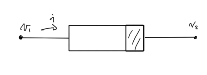
    Imagine, for example, that we have a component illustrated in fig. 1.

    fig. 1.  Variable voltage device

    fig. 1. Variable voltage device

    \begin{equation}\label{eqn:multiphysicsL4:20}
    v_1 – v_2 = 3 i^2
    \end{equation}

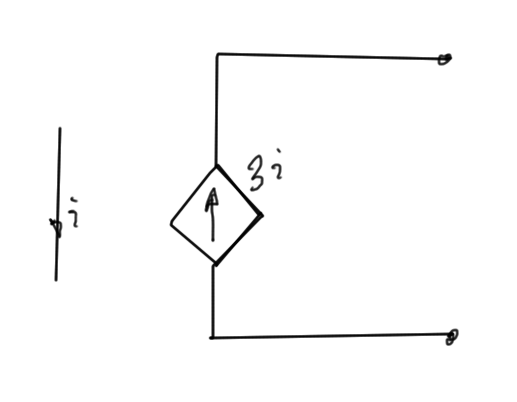
  • any current which is controlling dependent sources, as in fig. 2.
    fig. 2.  Current controlled device

    fig. 2. Current controlled device

  • Inductors
    \begin{equation}\label{eqn:multiphysicsL4:40}
    v_1 – v_2 = L \frac{di}{dt}.
    \end{equation}

Solving large systems

We are interested in solving linear systems of the form

\begin{equation}\label{eqn:multiphysicsL4:60}
M \overline{{x}} = \overline{{b}},
\end{equation}

possibly with thousands of elements.

Gaussian elimination

\begin{equation}\label{eqn:multiphysicsL4:80}
\begin{bmatrix}
M_{11} & M_{12} & M_{13} \\
M_{21} & M_{22} & M_{23} \\
M_{31} & M_{32} & M_{33} \\
\end{bmatrix}
\begin{bmatrix}
x_1 \\
x_2 \\
x_3 \\
\end{bmatrix}
=
\begin{bmatrix}
b_1 \\
b_2 \\
b_3 \\
\end{bmatrix}
\end{equation}

It’s claimed for now, to be seen later, that back substitution is the fastest way to arrive at the solution, less computationally complex than completion the diagonalization.

Steps

\begin{equation}\label{eqn:multiphysicsL4:100}
(1) \cdot \frac{M_{21}}{M_{11}} \Rightarrow
\begin{bmatrix}
M_{21} & \frac{M_{21}}{M_{11}} M_{12} & \frac{M_{21}}{M_{11}} M_{13} \\
\end{bmatrix}
\end{equation}

\begin{equation}\label{eqn:multiphysicsL4:120}
(2) \cdot \frac{M_{31}}{M_{11}} \Rightarrow
\begin{bmatrix}
M_{31} & \frac{M_{31}}{M_{11}} M_{32} & \frac{M_{31}}{M_{11}} M_{33} \\
\end{bmatrix}
\end{equation}

This gives

\begin{equation}\label{eqn:multiphysicsL4:140}
\begin{bmatrix}
M_{11} & M_{12} & M_{13} \\
0 & M_{22} – \frac{M_{21}}{ M_{11} } M_{12} & M_{23} – \frac{M_{21}}{M_{11}} M_{13} \\
0 & M_{32} – \frac{M_{31}}{M_{11}} M_{32} & M_{33} – \frac{M_{31}}{M_{11}} M_{33} \\
\end{bmatrix}
\begin{bmatrix}
x_1 \\
x_2 \\
x_3 \\
\end{bmatrix}
=
\begin{bmatrix}
b_1 \\
b_2 – \frac{M_{21}}{M_{11}} b_1 \\
b_3 – \frac{M_{31}}{M_{11}} b_1
\end{bmatrix}.
\end{equation}

Here the \( M_{11} \) element is called the {pivot}. Each of the \(
M_{j1}/M_{11} \) elements is called a {multiplier}. This operation can be written as

\begin{equation}\label{eqn:multiphysicsL4:160}
\begin{bmatrix}
M_{11} & M_{12} & M_{13} \\
0 & M_{22}^{(2)} & M_{23}^{(3)} \\
0 & M_{32}^{(2)} & M_{33}^{(3)} \\
\end{bmatrix}
\begin{bmatrix}
x_1 \\
x_2 \\
x_3 \\
\end{bmatrix}
=
\begin{bmatrix}
b_1 \\
b_2^{(2)} \\
b_3^{(2)} \\
\end{bmatrix}.
\end{equation}

Using \( M_{22}^{(2)} \) as the pivot this time, we form
\begin{equation}\label{eqn:multiphysicsL4:180}
\begin{bmatrix}
M_{11} & M_{12} & M_{13} \\
0 & M_{22}^{(2)} & M_{23}^{(3)} \\
0 & 0 & M_{33}^{(3)} – \frac{M_{32}^{(2)}}{M_{22}^{(2)}} M_{23}^{(2)} \\
\end{bmatrix}
\begin{bmatrix}
x_1 \\
x_2 \\
x_3 \\
\end{bmatrix}
=
\begin{bmatrix}
b_1 \\
b_2 – \frac{M_{21}}{M_{11}} b_1 \\
b_3 – \frac{M_{31}}{M_{11}} b_1
– \frac{M_{32}^{(2)}}{M_{22}^{(2)}} b_{2}^{(2)} \\
\end{bmatrix}.
\end{equation}

LU decomposition

Through Gaussian elimination, we have transformed the system from

\begin{equation}\label{eqn:multiphysicsL4:200}
M x = b
\end{equation}

to
\begin{equation}\label{eqn:multiphysicsL4:220}
U x = y.
\end{equation}

Writing out our Gaussian transformation in the form \( U \overline{{x}} = b \) we have

\begin{equation}\label{eqn:multiphysicsL4:240}
U \overline{{x}} =
\begin{bmatrix}
1 & 0 & 0 \\
-\frac{M_{21}}{M_{11}} & 1 & 0 \\
\frac{M_{32}^{(2)}}{M_{22}^{(2)}}
\frac{M_{21}}{M_{11}}

\frac{M_{31}}{M_{11}}
&

\frac{M_{32}^{(2)}}{M_{22}^{(2)}}
& 1
\end{bmatrix}
\begin{bmatrix}
b_1 \\
b_2 \\
b_3
\end{bmatrix}.
\end{equation}

We can verify that the operation matrix \( K^{-1} \), where \( K^{-1} U = M \) that takes us to this form is

\begin{equation}\label{eqn:multiphysicsL4:260}
\begin{bmatrix}
1 & 0 & 0 \\
\frac{M_{21}}{M_{11}} & 1 & 0 \\
\frac{M_{31}}{M_{11}} &
\frac{M_{32}^{(2)}}{M_{22}^{(2)}} &
1
\end{bmatrix}
\begin{bmatrix}
U_{11} & U_{12} & U_{13} \\
0 & U_{22} & U_{23} \\
0 & 0 & U_{33} \\
\end{bmatrix}
\overline{{x}} = \overline{{b}}
\end{equation}

Using this {LU} decomposition is generally superior to standard Gaussian elimination, since we can use this for many different \(\overline{{b}}\) vectors using the same amount of work.

Our steps are

\begin{equation}\label{eqn:multiphysicsL4:280}
b
= M x
= L \lr{ U x}
\equiv L y.
\end{equation}

We can now solve \( L y = b \), using substitution for \( y_1 \), then \( y_2 \), and finally \( y_3 \). This is called {forward substitution}.

Finally, we can now solve

\begin{equation}\label{eqn:multiphysicsL4:300}
U x = y,
\end{equation}

using {back substitution}.

Note that we produced the vector \( y \) as a side effect of performing the Gaussian elimination process.