[Click here for a PDF version of this post]
Motivation: explain field formulas in an engineering problem set.
The following equations were given in a problem set for the magnitude of the electric field strength at a point \( z \) due to symmetric ring and disk charge distributions respectively:
\begin{equation}\label{eqn:ringAndDiskField:20}
E = \frac{q z}{4 \pi \epsilon_0 \lr{ z^2 + R^2 }^{3/2} },
\end{equation}
\begin{equation}\label{eqn:ringAndDiskField:40}
E = \frac{\sigma}{2 \epsilon_0} \lr{ 1 – \frac{ z }{\sqrt{ z^2 + R^2 }} }.
\end{equation}
While these were given as black box results to use in a few superposition problems, there isn’t actually any magic required to find these, provided one knows how to perform some line and area integrals.
Electric field due to charge distributions.
Assuming that we are talking about stationary charges, we have only an electric field. Recall that the field, measured at a point \( \Bx \) for a single stationary point situated at point \( \Bx’ \) is
\begin{equation}\label{eqn:ringAndDiskField:60}
\BE(\Bx) = \inv{4 \pi \epsilon_0} \frac{ q \lr{ \Bx – \Bx’ }}{\Norm{\Bx – \Bx’}^3 }.
\end{equation}
If we want to find the field due to charges \( q_k \) at points \( \Bx_k \), then we just sum over all those charges
\begin{equation}\label{eqn:ringAndDiskField:80}
\BE(\Bx) = \inv{4 \pi \epsilon_0} \sum_k \frac{ q_k \lr{ \Bx – \Bx_k }}{\Norm{\Bx – \Bx_k}^3 }.
\end{equation}
This sum can be extended to a continuous charge density. If \( \rho(\Bx) \) represents the charge per unit volume situated at point \( \Bx \), then the field due to that continuous charge density is
\begin{equation}\label{eqn:ringAndDiskField:100}
\BE(\Bx) = \inv{4 \pi \epsilon_0} \int dV’ \frac{ \rho(\Bx’) \lr{ \Bx – \Bx’ }}{\Norm{\Bx – \Bx’}^3 }.
\end{equation}
Similarly, if \( \sigma(\Bx) \) represents the charge per unit area for at point \( \Bx \), then the field due to that continuous surface charge density is
\begin{equation}\label{eqn:ringAndDiskField:120}
\BE(\Bx) = \inv{4 \pi \epsilon_0} \int dA’ \frac{ \sigma(\Bx’) \lr{ \Bx – \Bx’ }}{\Norm{\Bx – \Bx’}^3 }.
\end{equation}
Finally, if \( \lambda(\Bx) \) represents the charge per unit length situated at point \( \Bx \), then the field due to that continuous linear charge density is
\begin{equation}\label{eqn:ringAndDiskField:140}
\BE(\Bx) = \inv{4 \pi \epsilon_0} \int dl’ \frac{ \lambda(\Bx’) \lr{ \Bx – \Bx’ }}{\Norm{\Bx – \Bx’}^3 }.
\end{equation}
At least theoretically, given any set of charge distributions, it’s just a matter of integration to find the corresponding electric field at any point. It happens that these integrals can be tricky, but we can get lucky when the charge configurations have special symmetries, as in the problem set formulas.
Ring charge distribution.
Let’s compute the electric field at a point along the axis of a ring charge distribution. I’ll use \( \setlr{ \Be_1, \Be_2, \Be_3 } \) to represent the standard basis direction vectors. We are considering the geometry of fig. 1.
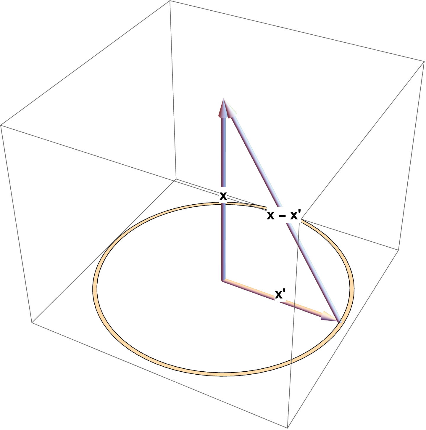
fig. 1. Circular ring charge distribution.
The point on the central axis can be written as
\begin{equation}\label{eqn:ringAndDiskField:160}
\Bx = z \Be_3,
\end{equation}
and the points on the ring are
\begin{equation}\label{eqn:ringAndDiskField:180}
\Bx'(\theta) = R \lr{ \Be_1 \cos\theta + \Be_2 \sin\theta },
\end{equation}
then
\begin{equation}\label{eqn:ringAndDiskField:200}
\Bx – \Bx’ = z \Be_3 – R \lr{ \Be_1 \cos\theta + \Be_2 \sin\theta },
\end{equation}
and
\begin{equation}\label{eqn:ringAndDiskField:220}
\Norm{\Bx – \Bx’}^2 = z^2 + R^2.
\end{equation}
Since \( R d\theta \) is the length of a segment of the ring, the charge on that segment is \( R d\theta \lambda \), and the field is
\begin{equation}\label{eqn:ringAndDiskField:240}
\begin{aligned}
\BE(\Bx)
&= \inv{4 \pi \epsilon_0} \int_{\theta =0}^{2 \pi} R d\theta \lambda \frac{z \Be_3 – R \lr{ \Be_1 \cos\theta + \Be_2 \sin\theta }}{\lr{ z^2 + R^2 }^{3/2} } \\
&= \inv{4 \pi \epsilon_0} \frac{2 \pi R z \Be_3 }{ \lr{ z^2 + R^2 }^{3/2} }.
\end{aligned}
\end{equation}
Observe that the integral of the \( \sin\theta \) and \( \cos\theta \) components are zero, since we are integrating over a full period. Finally, since the total charge is \( q = 2 \pi R \lambda \), we have
\begin{equation}\label{eqn:ringAndDiskField:260}
\BE(0, 0, z) = \inv{4 \pi \epsilon_0} \frac{q z \Be_3 }{ \lr{ z^2 + R^2 }^{3/2} }.
\end{equation}
This recovers the equation from the problem set, with the only difference being the explicit inclusion of the direction vector, which was implied in the problem statement.
Field of a disk.
The setup above can be used to state the integral to solve for the field of a disk. The area of a segment of the disk is \( r dr d\theta \), so the charge of that fragment is \( r dr d\theta \sigma \), so the field is
\begin{equation}\label{eqn:ringAndDiskField:280}
\begin{aligned}
\BE(\Bx)
&= \inv{4 \pi \epsilon_0} \int_{r = 0}^R \int_{\theta =0}^{2 \pi} r dr d\theta \sigma \frac{z \Be_3 – r \lr{ \Be_1 \cos\theta + \Be_2 \sin\theta }}{\lr{ z^2 + r^2 }^{3/2} } \\
&= \frac{\sigma z \Be_3}{2 \epsilon_0} \int_{r = 0}^R dr \frac{r}{\lr{ z^2 + r^2 }^{3/2} }.
\end{aligned}
\end{equation}
As before, when evaluating the \( \theta \) integral, the sinusoidal components are killed. Since \( \int_0^{2 \pi} d\theta = 2 \pi \), we have a nice cancellation of \( 2 \pi \) downstairs.
Finally, provided \( z \ne 0 \),
\begin{equation}\label{eqn:ringAndDiskField:300}
\int_{r = 0}^R dr \frac{r}{\lr{ z^2 + r^2 }^{3/2} } = \inv{\Abs{z}} – \inv{\sqrt{ z^2 + R^2 }},
\end{equation}
so the electric field is
\begin{equation}\label{eqn:ringAndDiskField:320}
\BE(0, 0, z) = \frac{ \sigma }{2 \epsilon_0 } \lr{ \mathrm{sgn}(z) – \frac{z}{\sqrt{z^2 + R^2}} },
\end{equation}
where \( \mathrm{sgn}(z) \) is the sign of \( z \). We see that the equation provided in the problem set is actually only true for \( z > 0 \), and needs a sign correction otherwise.