This is a continuation of:
[Click here for a PDF of these posts with colored equations, and additional figures and commentary]
Vectors.
Cast yourself back in time, all the way to high school, where the first definition of vector that you would have encountered was probably very similar to the one made famous by the not very villainous Vector in Despicable Me [4]. His definition was not complete, but it is a good starting point:
Definition: Vector. A vector is a quantity represented by an arrow with both direction and magnitude.
All the operations that make vectors useful are missing from this definition, such as
- a comparison operator,
- a rescaling operation (i.e. a scalar multiplication operation that changes the length),
- addition and subtraction operators,
- an operator that provides the length of a vector,
- multiplication or multiplication like operations.
The concept of vector, once supplemented with the operations above, will be useful since it models many directed physical quantities that we experience daily. These include velocity, acceleration, forces, and electric and magnetic fields.
Vector comparison.
In fig. 1.1 (a), we have three vectors, labelled \( \Ba, \Bb, \Bc \), all with different directions and magnitudes, and in fig. 1.1 (b), those vectors have each been translated (moved without rotation or change of length) slightly. Two vectors are considered equal if they have the same direction and magnitude. That is, two vectors are equal if one is the image of the other after translation. In these figures \( \Ba \ne \Bb, \Bb \ne \Bc, \Bc \ne \Ba \), whereas any same colored vectors are equal.
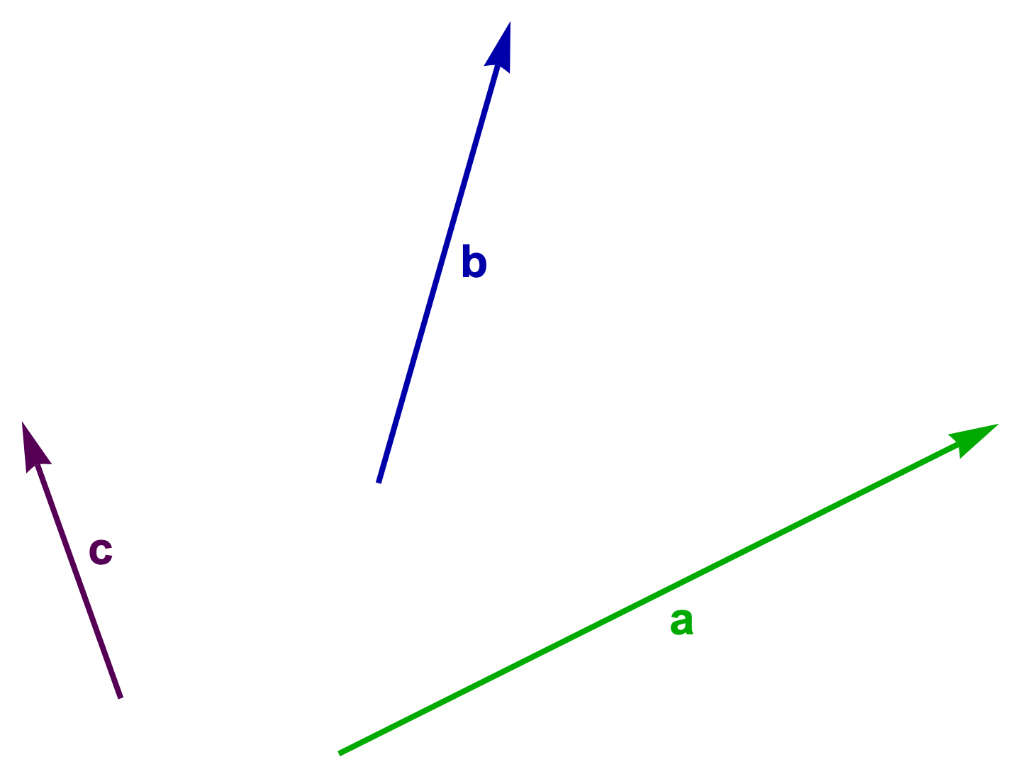
Figure 1.1 (a): Three vectors
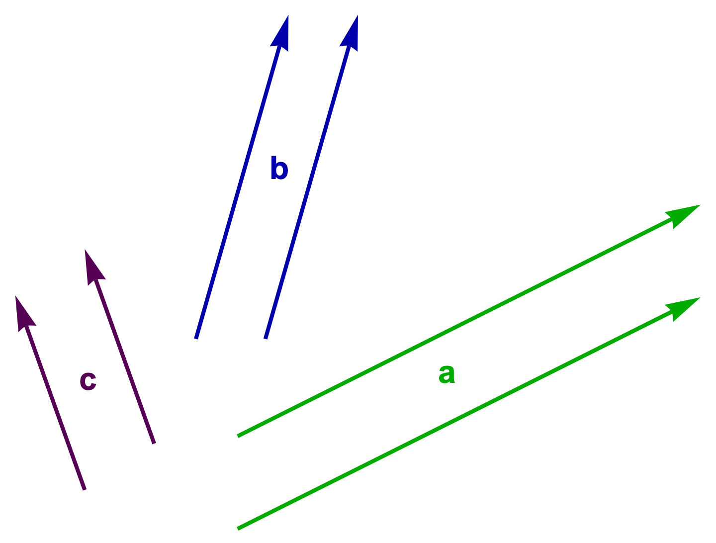
Figure 1.1 (b): Example translations of three vectors.
Vector (scalar) multiplication.
We can multiply vectors by scalars by changing their lengths appropriately.
In this context a scalar is a real number (this is purposefully vague, as it will be useful to allow scalars to be complex valued later.)
Using the example vectors, some rescaled vectors include \( 2 \Ba, (-1) \Bb, \pi \Bc \), as illustrated in fig. 1.2.
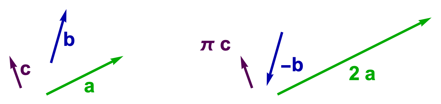
Figure. 1.2 Scaled vectors.
Vector addition.
Scalar multiplication implicitly provides an algorithm for addition of vectors that have the same direction, as \( s \Bx + t \Bx = (s+t) \Bx \) for any scalars \( s, t \). This is illustrated in fig. 1.3 where \( 2 \Ba = \Ba + \Ba \) is formed in two equivalent forms. We see that the addition of two vectors that have the same direction requires lining up those vectors head to tail. The sum of two such vectors is the vector that can be formed from the first tail to the final head.
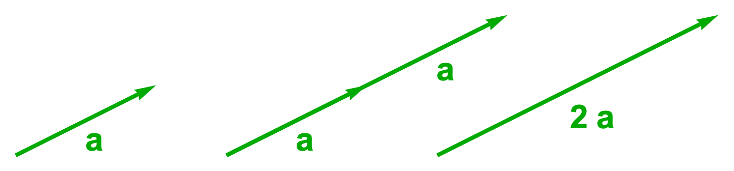
Figure 1.3. Twice a vector.
It turns out that this arrow daisy chaining procedure is an appropriate way of defining addition for any vectors.
Definition: Vector addition. The sum of two vectors can be found by connecting those two vectors head to tail in either order. The sum of the two vectors is the vector that can be formed by drawing an arrow from the initial tail to the final head. This can be generalized by chaining any number of vectors and joining the initial tail to the final head.
This addition procedure is illustrated in fig. 1.4, where \( \Bs = \Ba + \Bb + \Bc \) has been formed.
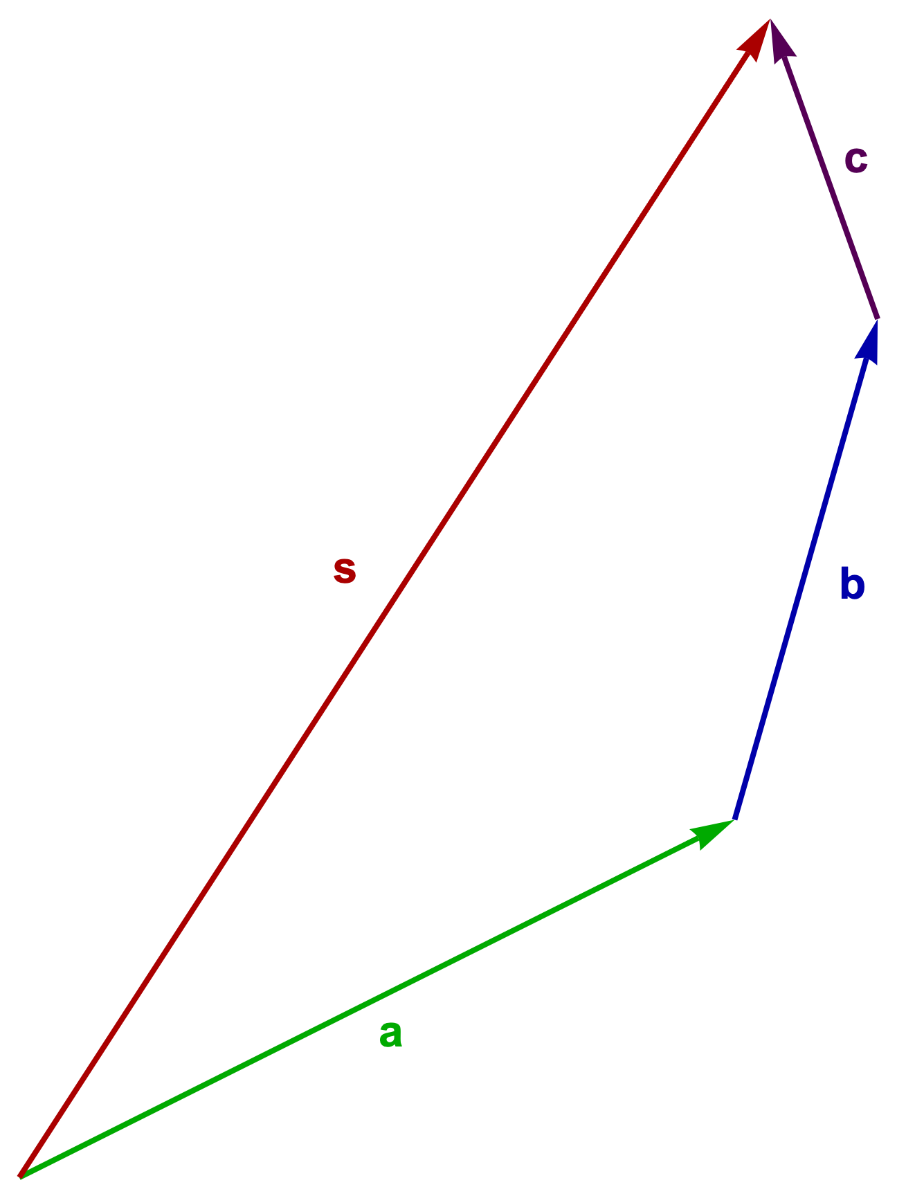
Figure 1.4. Addition of vectors.
This definition of vector addition was inferred from the observation of the rules that must apply to addition of vectors that lay in the same direction (colinear vectors). Is it a cheat to just declare that this rule for addition of colinear vectors also applies to arbitrary vectors? Yes, it probably is, but it’s a cheat that works nicely, and one that models physical quantities that we experience daily (velocities, acceleration, force, …). If you collect two friends you can demonstrate the workability of this inferred rule easily, by putting your arms out, and having your friends pull on them. If you put your arms opposing to the sides, and have your friends pull with equal forces, you’ll see that the force that can be represented by the pulling of your friends add to zero. If one of your friends is stronger, you’ll move more in that direction. If you put your arms out at 45 degree angles, you’ll see that you move along the direction of the sum of the forces. These scenarios are crudely sketched below in figure 1.x
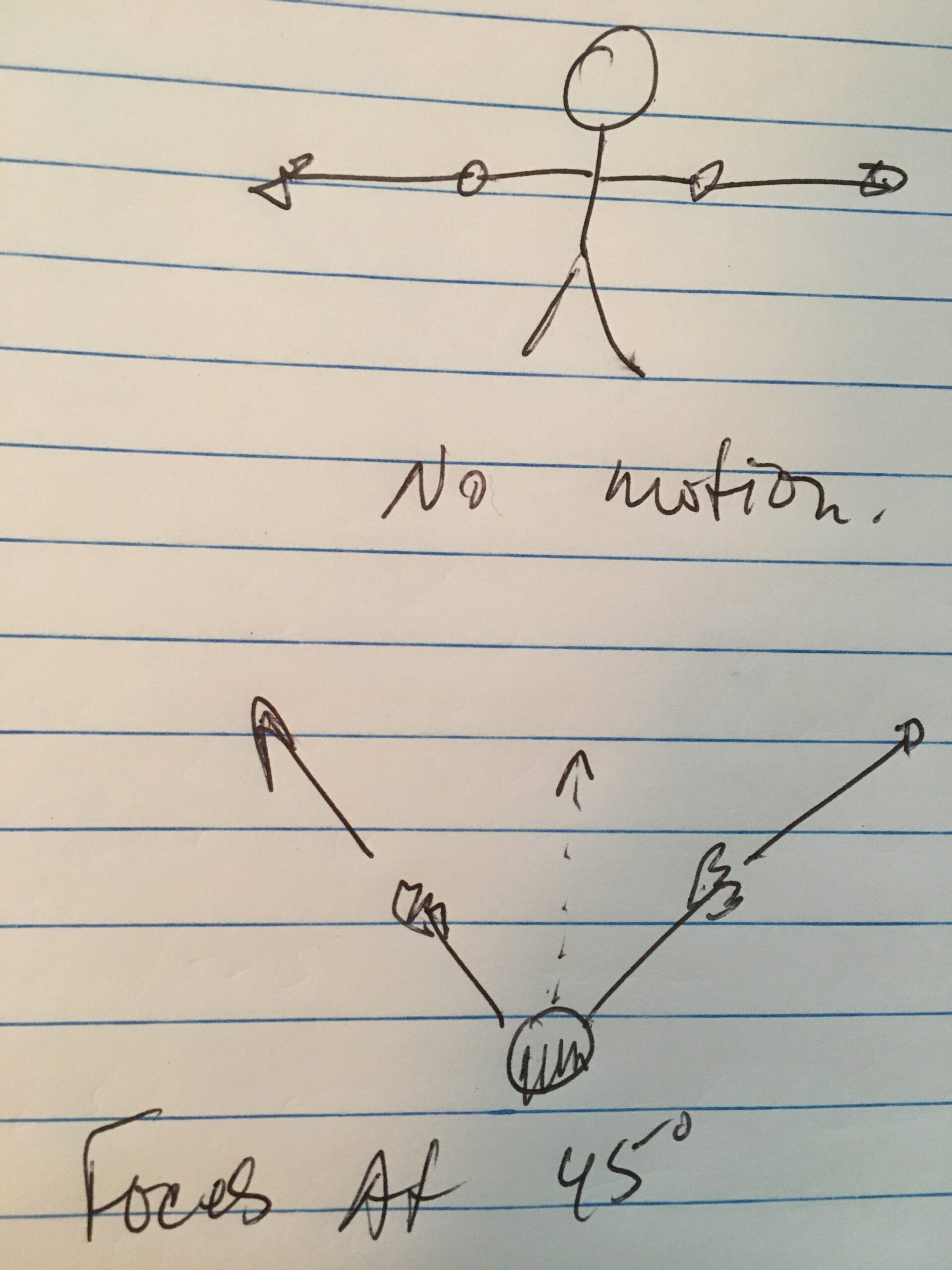
Figure 1.x: Friends pulling on your arms.
Vector subtraction.
Since we can scale a vector by \( -1 \) and we can add vectors, it is clear how to define vector subtraction
Definition: Vector subtraction. The difference of vectors \( \Ba, \Bb \) is
\begin{equation*}
\Ba – \Bb \equiv \Ba + ((-1)\Bb).
\end{equation*}
Graphically, subtracting a vector from another requires flipping the direction of the vector to be subtracted (scaling by \(-1\)), , and then adding both head to tail. This is illustrated in fig. 1.5.
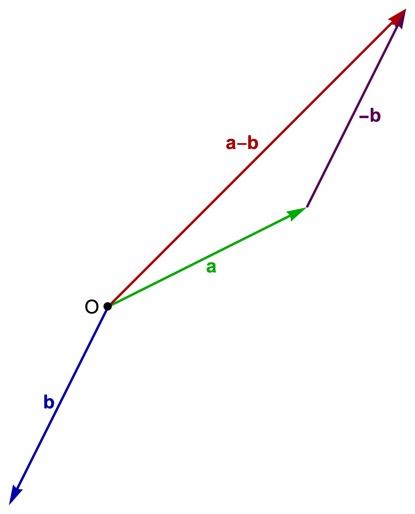
Figure 1.5. Vector subtraction.
Length and what’s to come.
It is easy to compute the length of a vector that has an arrow representation.
One simply lines a ruler of appropriate units along the vector and measures.
We actually want an algebraic way of computing length, but there is some baggage required, including
- Coordinates.
- Bases (plural of basis).
- Linear dependence and independence.
- Dot product.
- Metric.
The next part of this series will cover these topics. Our end goal is geometric algebra, which allows for many coordinate free operations, but we still have to use coordinates, both to read the literature, and in practice. Coordinates and non-orthonormal bases are also a good way to introduce non-Euclidean metrics.
References
[4] Vector; supervillain extraordinaire (Despicable Me). A quantity represented by an arrow with direction and magnitude. Youtube. URL https://www.youtube.com/watch?v=bOIe0DIMbI8. [Online; accessed 11-July-2020].
Mr. Joot, where is the next part of this series?
If there is one, I can’t find it and I would really appreciate it if you would let me know. Thank you,
– Frank
Hi Frank,
I’m going to have to search my computer and see if I did anything further as I had initially planned. In the interim, you might want to check out: https://peeterjoot.com/writing/geometric-algebra-for-electrical-engineers/ — that has all the raw material I planned to treat in this series, but I was hoping to produce something more palatable a 2nd time through.
Peeter