[Click here for a PDF version of this post]
Motivation.
On vacation I was reading some more of [1]. It was mentioned in passing that the area contained within a closed parameterized curve is given by
\begin{equation}\label{eqn:containedArea:20}
A = \inv{2} \int_{t_0}^{t_1} \lr{x y’ – y x’} dt,
\end{equation}
where \( x = x(t), y = y(t), t \in [t_0, t_1] \). This has the look of a Stokes theorem coordinate expansion (specifically, the Green’s theorem special case of Stokes’), but with somewhat mysterious looking factor of one half out in front. My aim in this post is to understand the origins of this area relationship, and play with it a bit.
Circular coordinates example.
The book suggests that the reader verify this for a circular parameterization, so we’ll do that here too.
Let
\begin{equation}\label{eqn:containedArea:40}
\begin{aligned}
x(t) &= r \cos t \\
y(t) &= r \sin t,
\end{aligned}
\end{equation}
where \( t \in [0, 2 \pi] \). Plugging in this, we have
\begin{equation}\label{eqn:containedArea:60}
\begin{aligned}
A
&= \inv{2} \int_0^{2 \pi} \lr{ r \cos t \lr{ r \cos t } – r \sin t \lr{ – r \sin t } } dt \\
&= \frac{r^2}{2} \int_0^{2 \pi} \lr{ \cos^2 t + \sin^2 t } dt \\
&= \frac{2 \pi r^2}{2} \\
&= \pi r^2.
\end{aligned}
\end{equation}
This simple example works out.
Piecewise linear parametrization example.
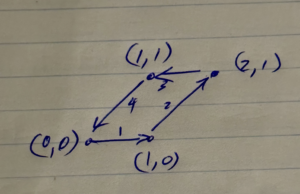
One parameterization of the unit parallelogram depicted in fig. 1 is
\begin{equation}\label{eqn:containedArea:340}
\begin{aligned}
(x,y) &= (t, 0),\quad t \in [0,1] \\
&= (t, t – 1),\quad t \in [1,2] \\
&= (4 – t, 1),\quad t \in [2,3] \\
&= (4 – t, 4 – t),\quad t \in [3,4]
\end{aligned}
\end{equation}
Respective evaluating of \( x y’ – y x’ \) in each of these regions gives
\begin{equation}\label{eqn:containedArea:360}
\begin{aligned}
(t) (0) – (0)(0) &= 0 \\
(t) (1) – (t-1)(1) &= 1 \\
(4-t)(0) – (1)(-1) &= 1 \\
(4-t)(-1) – (4-t)(-1) &= 0,
\end{aligned}
\end{equation}
and integrating
\begin{equation}\label{eqn:containedArea:380}
\inv{2} \int_0^4 \lr{ x y’ – y x’} dt = \frac{2}{2} = 1,
\end{equation}
as expected. In this example, the directional derivative is not continuous at the corners of the parallelogram, but that is not a requirement (as it should not be, as the area is well defined despite any corners.)
Can we discover this relationship using the Jacobian?
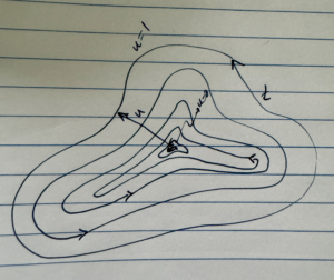
Graphically, I can imagine that we could find this area relationship, by considering a parameterization of a family of nested closed curves, as depicted in fig. 2.
For such a parameterization, calculating the area is just a Jacobian evaluation
\begin{equation}\label{eqn:containedArea:80}
\begin{aligned}
A
&= \iint \frac{\partial(x, y)}{\partial(u,t)} du dt \\
&= \iint \lr{ \PD{u}{x} \PD{t}{y} – \PD{u}{y} \PD{t}{x} } du dt \\
&= \iint \lr{ \PD{u}{x} y’ – \PD{u}{y} x’ } du dt.
\end{aligned}
\end{equation}
Let’s try to eliminate the \( u \) derivatives using integration by parts, and see what we get.
\begin{equation}\label{eqn:containedArea:100}
\begin{aligned}
A
&= \iint \lr{ \PD{u}{x} y’ – \PD{u}{y} x’ } du dt \\
&= \iint \frac{d}{du} \lr{ x y’ – y x’ } du dt – \iint \lr{ x \PD{u}{y’} – y \PD{u}{x’} } du dt \\
&= \int \lr{ x y’ – y x’ } dt – \iint \lr{ x \PD{u}{y’} – y \PD{u}{x’} } du dt.
\end{aligned}
\end{equation}
This is interesting, as we find the area equation that we are interested (times two), but we have a strange new area equation. Essentially, we have found, assuming we trust the claim in the book, that
\begin{equation}\label{eqn:containedArea:120}
A = 2 A – \iint \lr{ x \PD{u}{y’} – y \PD{u}{x’} } du dt,
\end{equation}
so it seems that the area can also be expressed as
\begin{equation}\label{eqn:containedArea:140}
A = \iint \lr{ x \frac{\partial^2 y}{\partial u \partial t} – y \frac{\partial^2 x}{\partial u \partial t} } du dt.
\end{equation}
Let’s again use the circular parameterization to verify that this works. I won’t try to prove this directly, but instead, we’ll use Stokes’ theorem to prove the stated result, from which we get this second derivative area formula as a side effect by virtue of our integration by parts expansion above.
For the circular parameterization, we have
\begin{equation}\label{eqn:containedArea:160}
\begin{aligned}
A
&= \int_{r = 0}^R dr \int_{t = 0}^{2 \pi} dt \lr{ x \frac{\partial^2 y}{\partial r \partial t} – y \frac{\partial^2 x}{\partial r \partial t} } \\
&= \int_{r = 0}^R dr \int_{t = 0}^{2 \pi} dt \lr{ r \cos t \frac{\partial \sin t}{\partial t} – r \sin t \frac{\partial \cos t}{\partial t} } \\
&= \int_{r = 0}^R r dr \int_{t = 0}^{2 \pi} dt \lr{ \cos^2 t + \sin^2 t } \\
&= \frac{R^2}{2} 2 \pi \\
&= \pi R^2.
\end{aligned}
\end{equation}
This checks out, at least for this one specific circular parameterization.
Area formula derivation using Stokes’ theorem.
Theorem 1.1: Green’s theorem.
\iint dx dy \lr{ \PD{x}{M} – \PD{y}{L} } = \oint L dx + M dy.
\end{equation}
Start proof:
We start with the general two parameter integration theorem
\begin{equation}\label{eqn:containedArea:180}
\iint F d^2 \Bx \lrpartial G = -\oint F d\Bx G,
\end{equation}
set \( F = 1, G = \Bf \), and apply scalar selection
\begin{equation}\label{eqn:containedArea:200}
\iint \gpgradezero{ d^2 \Bx \lrpartial \Bf } = -\oint d\Bx \cdot \Bf,
\end{equation}
to find the two parameter form of Stokes’ theorem
\begin{equation}\label{eqn:containedArea:220}
\iint d^2 \Bx \cdot \lr{ \spacegrad \wedge \Bf } = -\oint d\Bx \cdot \Bf,
\end{equation}
With a planar parameterization, say \( \Bf = L \Be_1 + M \Be_2 \), we have \( d\Bx \cdot \Bf = L dx + M dy \), and for the LHS
\begin{equation}\label{eqn:containedArea:240}
\begin{aligned}
\iint d^2 \Bx \cdot \lr{ \spacegrad \wedge \Bf }
&=
\iint dx dy \Be_{12}^2
\begin{vmatrix}
\partial_1 & \partial_2 \\
L & M
\end{vmatrix} \\
&=
-\iint dx dy \lr{ \PD{x}{M} – \PD{y}{L} }.
\end{aligned}
\end{equation}
End proof.
Parameterized area equation.
If we wish to evaluate an elementary area, we can pick \( L, M \) such that \( \PDi{x}{M} – \PDi{y}{L} = 1 \). One such selection is
\begin{equation}\label{eqn:containedArea:280}
\begin{aligned}
M &= \frac{x}{2} \\
L &= -\frac{y}{2},
\end{aligned}
\end{equation}
so
\begin{equation}\label{eqn:containedArea:300}
A = \inv{2} \oint -y dx + x dy = \inv{2} \int \lr{ x y’ – y x’ } dt.
\end{equation}
Clearly, there are other possible choices of \( L, M \) that we could use to find alternate area equations, but this choice seems to be independent of the shape of the region.
References
[1] F.W. Byron and R.W. Fuller. Mathematics of Classical and Quantum Physics. Dover Publications, 1992.

