[Click here for a PDF of this post with nicer formatting]
Disclaimer
Peeter’s lecture notes from class. These may be incoherent and rough.
Assembling system equations automatically. Node/branch method
Consider the sample circuit of fig. 1.
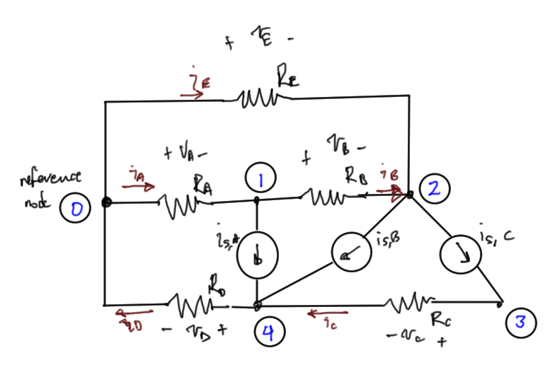
fig. 1. Sample resistive circuit
Step 1. Choose unknowns:
For this problem, let’s take
- node voltages: \(V_1, V_2, V_3, V_4\)
- branch currents: \(i_A, i_B, i_C, i_D, i_E\)
We do not need to introduce additional labels for the source current sources.
We always introduce a reference node and call that zero.
For a circuit with \(N\) nodes, and \(B\) resistors, there will be \(N-1\) unknown node voltages and \(B\) unknown branch currents, for a total number of \(N – 1 + B\) unknowns.
Step 2. Conservation equations:
KCL
- 0: \(i_A + i_E – i_D = 0\)
- 1: \(-i_A + i_B + i_{S,A} = 0\)
- 2: \(-i_B + i_{S,B} – i_E + i_{S,C} = 0\)
- 3: \(i_C – i_{S,C} = 0\)
- 4: \(-i_{S,A} – i_{S,B} + i_D – i_C = 0\)
Grouping unknown currents, this is
- 0: \(i_A + i_E – i_D = 0\)
- 1: \(-i_A + i_B = -i_{S,A}\)
- 2: \(-i_B -i_E = -i_{S,B} -i_{S,C}\)
- 3: \(i_C = i_{S,C}\)
- 4: \(i_D – i_C = i_{S,A} + i_{S,B}\)
Note that one of these equations is redundant (sum 1-4). In a circuit with \(N\) nodes, we can write at most \(N-1\) independent KCLs.
In matrix form
\begin{equation}\label{eqn:multiphysicsL2:20}
\begin{bmatrix}
-1 & 1 & 0 & 0 & 0 \\
0 & -1 & 0 & 0 & -1 \\
0 & 0 & 1 & 0 & 0 \\
0 & 0 & -1 & 1 & 0
\end{bmatrix}
\begin{bmatrix}
i_A \\
i_B \\
i_C \\
i_D \\
i_E \\
\end{bmatrix}
=
\begin{bmatrix}
-i_{S,A} \\
-i_{S,B} -i_{S,C} \\
i_{S,C} \\
i_{S,A} + i_{S,B}
\end{bmatrix}
\end{equation}
We call this first matrix of ones and minus ones the incidence matrix \(A\). This matrix has \(B\) columns and \(N-1\) rows. We call the known current matrix \(\overline{I}_S\), and the branch currents \(\overline{I}_B\). That is
\begin{equation}\label{eqn:multiphysicsL2:40}
A \overline{I}_B = \overline{I}_S.
\end{equation}
Observe that we have both a plus and minus one in all columns except for those columns impacted by our neglect of the reference node current conservation equation.
Algorithm for filling \(A\)
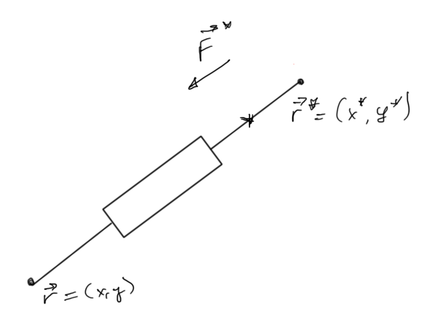
In the input file, to describe a resistor of fig. 2, you’ll have a line of the form
R name \(n_1\) \(n_2\) value
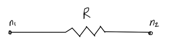
fig. 2. Resistor node convention
The algorithm to process resistor lines is
\begin{equation*}
\begin{aligned}
&A \leftarrow 0 \\
&ic \leftarrow 0 \\
&\text{forall resistor lines} \\
&ic \leftarrow ic + 1, \text{adding one column to \(A\)} \\
&\text{if}\ n_1 != 0 \\
&A(n_1, ic) \leftarrow +1 \\
&\text{endif} \\
&\text{if}\ n_2 != 0 \\
&A(n_2, ic) \leftarrow -1 \\
&\text{endif} \\
&\text{endfor} \\
\end{aligned}
\end{equation*}
Algorithm for filling \(\overline{I}_S\)
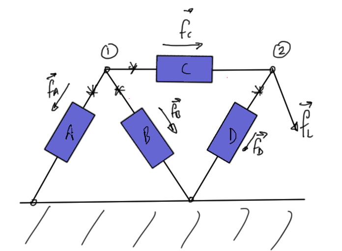
Current sources, as in fig. 3, a line will have the specification (FIXME: confirm… didn’t write this down).
I name \(n_1\) \(n_2\) value
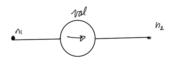
fig. 3. Current source conventions
\begin{equation*}
\begin{aligned}
&\overline{I}_S = \text{zeros}(N-1, 1) \\
&\text{forall current lines} \\
&\overline{I}_S(n_1) \leftarrow \overline{I}_S(n_1) – \text{value} \\
&\overline{I}_S(n_2) \leftarrow \overline{I}_S(n_1) + \text{value} \\
&\text{endfor}
\end{aligned}
\end{equation*}
Step 3. Constitutive equations:
\begin{equation}\label{eqn:multiphysicsL2:60}
\begin{bmatrix}
i_A \\
i_B \\
i_C \\
i_D \\
i_E
\end{bmatrix}
=
\begin{bmatrix}
1/R_A & & & & \\
& 1/R_B & & & & \\
& & 1/R_C & & & \\
& & & 1/R_D & & \\
& & & & & 1/R_E
\end{bmatrix}
\begin{bmatrix}
v_A \\
v_B \\
v_C \\
v_D \\
v_E
\end{bmatrix}
\end{equation}
Or
\begin{equation}\label{eqn:multiphysicsL2:80}
\overline{I}_B = \alpha \overline{V}_B,
\end{equation}
where \(\overline{V}_B\) are the branch voltages, not unknowns of interest directly. We can write
\begin{equation}\label{eqn:multiphysicsL2:100}
\begin{bmatrix}
v_A \\
v_B \\
v_C \\
v_D \\
v_E
\end{bmatrix}
=
\begin{bmatrix}
-1 & & & \\
1 & -1 & & \\
& & 1 & -1 \\
& & & 1 \\
& -1 & &
\end{bmatrix}
\begin{bmatrix}
v_1 \\
v_2 \\
v_3 \\
v_4
\end{bmatrix}
\end{equation}
Observe that this is the transpose of \(A\), allowing us to write
\begin{equation}\label{eqn:multiphysicsL2:120}
\overline{V}_B = A^\T \overline{V}_N.
\end{equation}
Solving
- KCLs: \(A \overline{I}_B = \overline{I}_S\)
- constitutive: \(\overline{I}_B = \alpha \overline{V}_B \Rightarrow \overline{I}_B = \alpha A^\T \overline{V}_N\)
- branch and node voltages: \(\overline{V}_B = A^\T \overline{V}_N\)
In block matrix form, this is
\begin{equation}\label{eqn:multiphysicsL2:140}
\begin{bmatrix}
A & 0 \\
I & -\alpha A^\T
\end{bmatrix}
\begin{bmatrix}
\overline{I}_B \\
\overline{V}_N
\end{bmatrix}
=
\begin{bmatrix}
\overline{I}_S \\
0
\end{bmatrix}.
\end{equation}
Is it square? We see that it is after observing that we have
- \(N-1\) rows in \(A\) , and \(B\) columns.
- \(B\) rows in \(I\).
- \(N-1\) columns.