For most of the time that I was at IBM (before leaving to LzLabs), I was enrolled in the Employee Charitable Fund (ECF) program. The ECF was a really easy way to do charitable donations, as the donations were small biweekly payroll deductions. As all the charitable options were official Canadian charities, I also got that tiny little tax deduction kickback as well.
Despite those benefits, I never really liked the ECF charity options, as it felt like my money was just going into a black hole. I heard about Kiva on the “How things work” podcast, and decided to bail from the ECF for a while and make some Kiva loans instead. Kiva is a microloan service, where you can loan selected individuals money in $25 increments. You get to pick who you want to loan to. As you get paid back, you can funnel those funds back into new loans.
Switching my funds to Kiva loans isn’t a charitable donation in the traditional sense. In particular, it doesn’t count as an offical Canadian charitable, so I don’t get any tax kickbacks. Those are usually just pennies anyways, so that’s not a big loss. If you are in the US you can get a tax kickback for donations to Kiva itself, but not for your loans. However, I treat my Kiva account like it’s a one way donation, funneling money in, and recycling all of it into new loans when I get payments.
In a rather timely fashion, as it’s was my end of month “Kiva donation time”, I got a notification of leanpub royalties today:
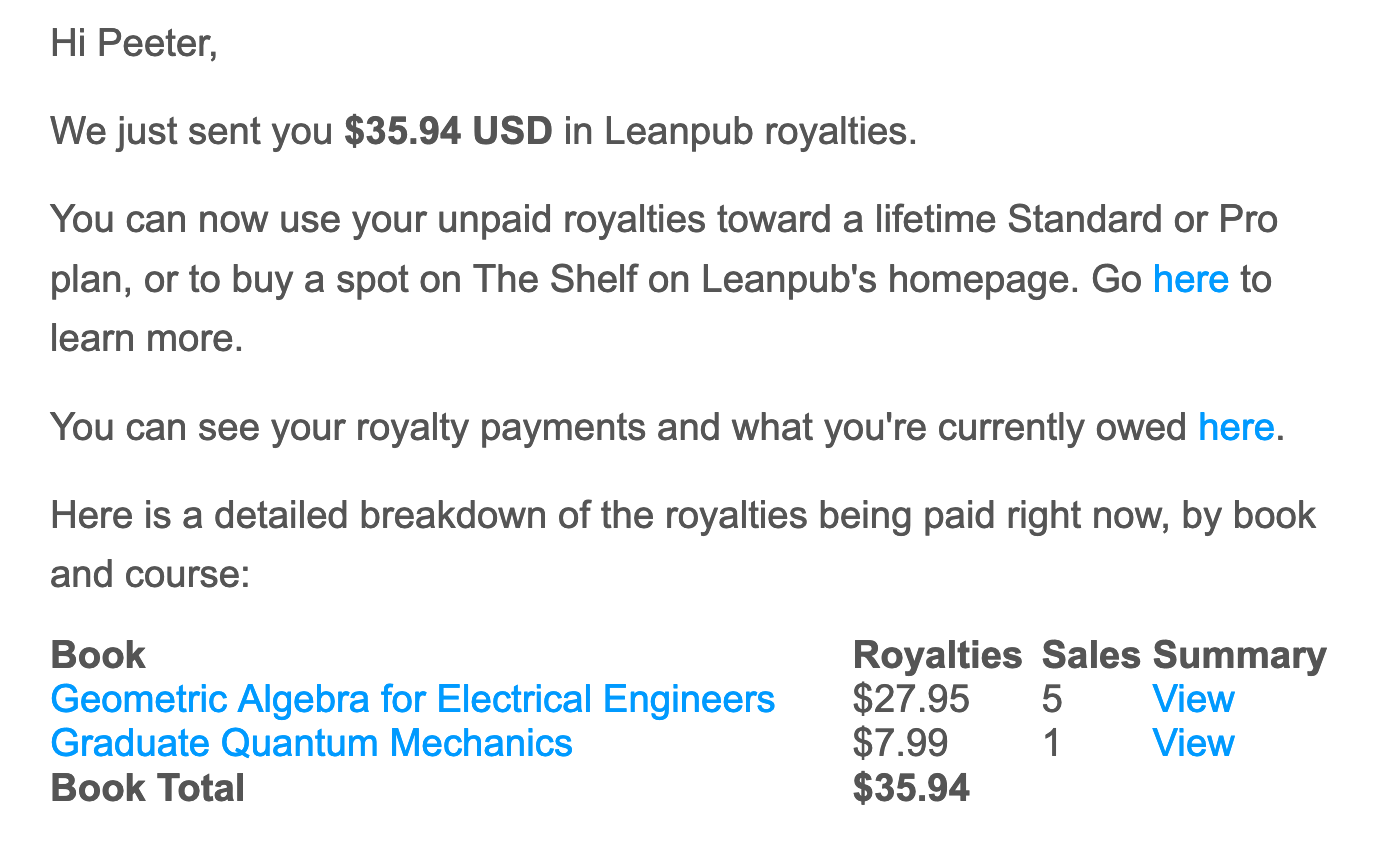
Leanpub is a pay what you want e-book publishing service that provides the purchasers with automatic updates, and purchaser only forums for Q&A. I didn’t really expect anybody would buy my stuff on leanpub, since I also make pdfs of all those books available for free. However, I don’t feel guilty about that for a couple reasons. One is that the purchaser has freedom to pick their price, and most seem to go over minimum. The other reason is that I have been funneling my leanpub royalties when I get them into my Kiva account. Usually, y leanpub sales, as they are batched and sporadic, don’t cover my regular Kiva contributions, but this month, they did.
Having been making kiva loans and contributions for so many years now, I’ve got a pretty decent distribution of countries covered:
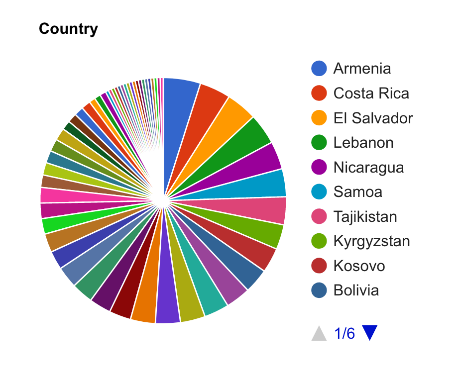
I regularly reset my ‘Saved Search’ to remove the most frequently leant to countries, and it looks like it’s time to do that again.
I’m pretty selective about the categories that I select my microloans, and that bias is obvious looking at the distribution of the loan categories I’ve selected:
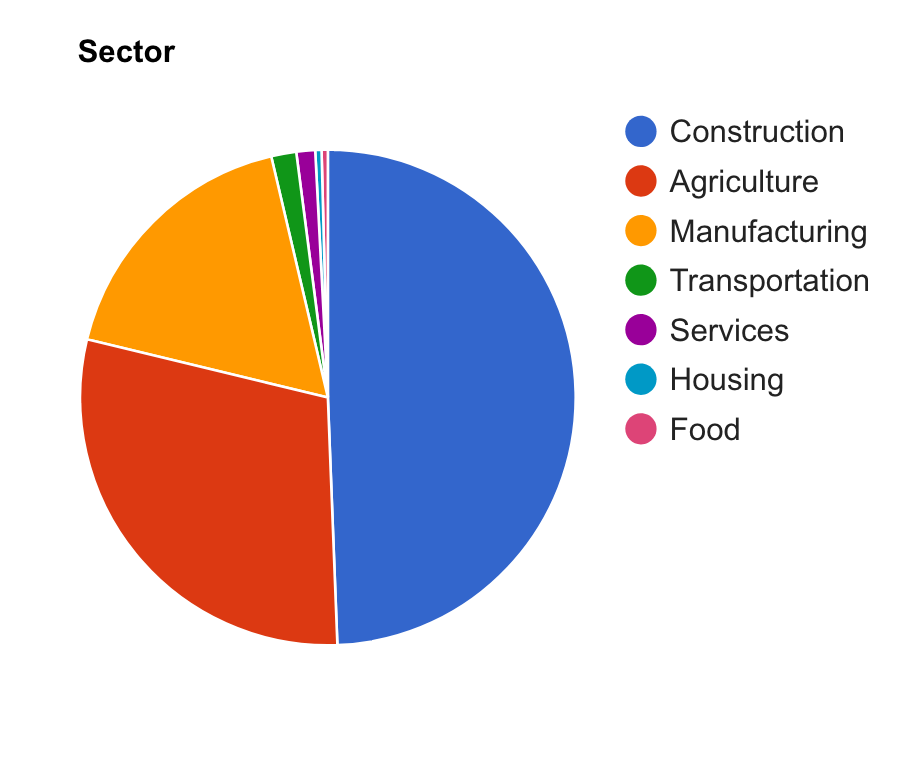
I particularly like the construction loan category, since I can pick somebody looking for tools to improve their business. I like the self sustainability of that.
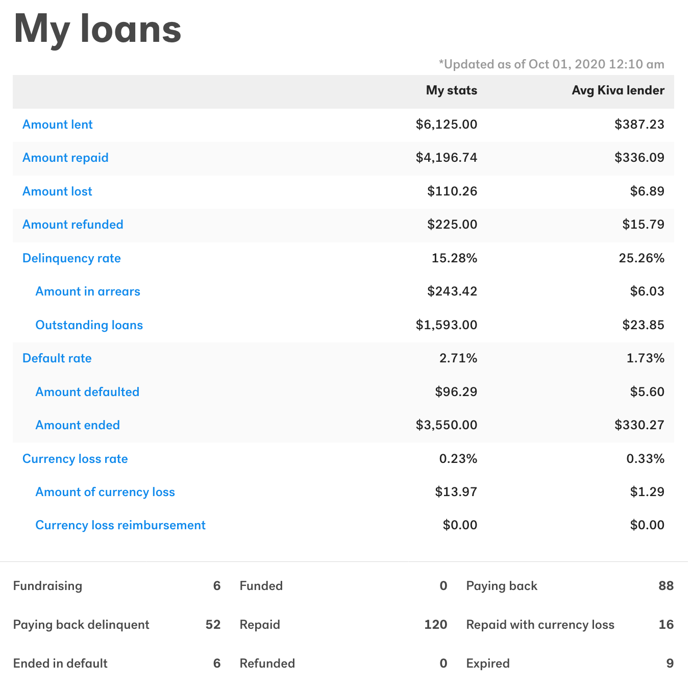
This strategy of small regular loans that feed back on themselves really accumulates nicely. I’ve been making only small monthly contributions, yet that has added up to $6K of total loans over the years, and I’ve now got $1500 of loans in the pipe. I’ve lost only about $100, which compared to the management fees of a typical charity, is actually pretty extraordinary. I’ve also lost a small amounts to donations to Kiva itself. They are asking for lots per loan these days, and I cheap out those contributions, but that has probably still added up.