It turns out, like GDB, that lldb has a TUI mode too, but it’s really simplistic. You enter with
(lldb) gui
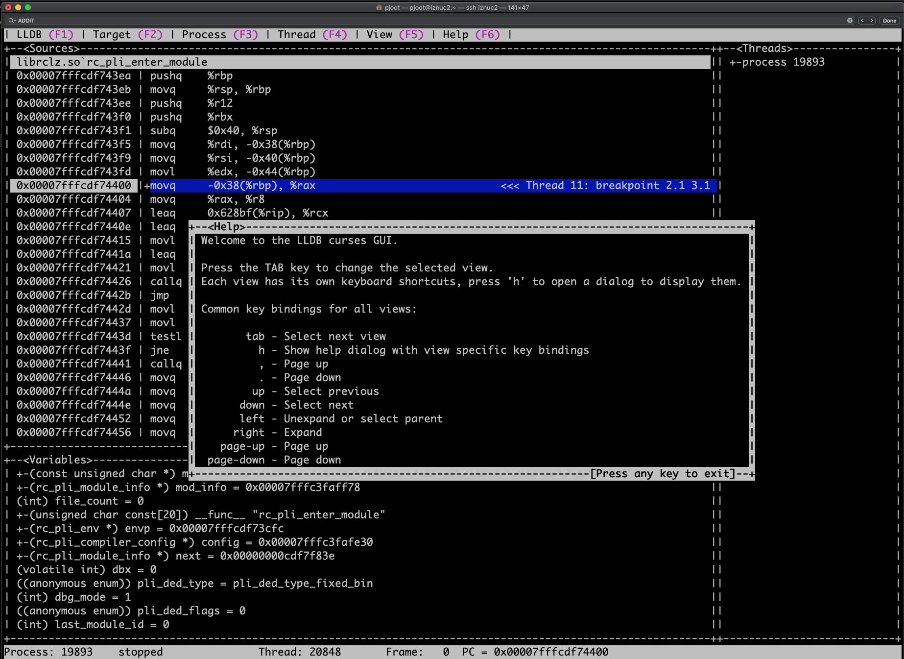
at which point you get a full screen of code or assembly, and options for register exploration, thread and stack exploration, and a variable view. The startup screen looks like:
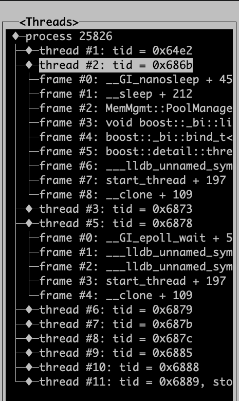
If you tab over to the Threads window, you can space select the process, and drill into the stack traces for any of the running threads
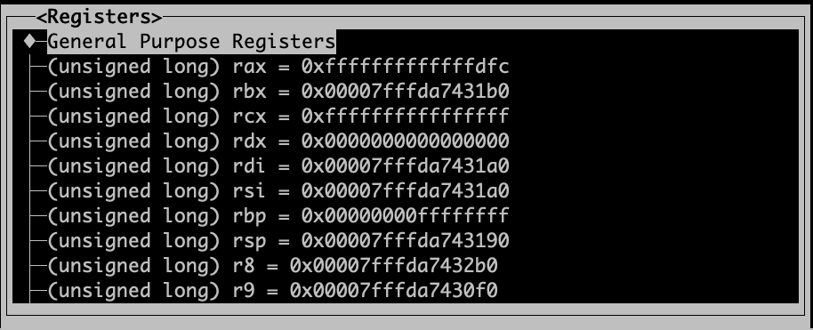
You can also expand the regsiters by register class:
I’d like to know how to resize the various windows. If you resize the terminal, the size of the stack view pane seems to remain fixed, so the symbol names always end up truncated.
Apparently this code hasn’t been maintained or developed since it was added. Because there is no console pane, you have to set all desired breakpoints and continue, then pop into the GUI to look at stuff, and then <F1> to get back to the console prompt. It’s nice that it gives you a larger view of the code, but given that lldb already displays context around each line, the lldb TUI isn’t that much of a value add in that respect.
This “GUI” would actually be fairly usable if it just had a console pane.