


The following was a rough outline for some words I said at Mom’s service.
Mom always seemed a lot like an unstoppable force. Anybody that knew her would probably agree, so a sudden diagnosis of cancer came as a shock to us all. It’s still hard to believe. Even with her body treasonously shutting down, mom wasn’t finished living, and was making long term plans. Those plans including continuing her roles as mother, grandmother, musician, and wife. It looks like Mom will have to defer and change some of her plans.
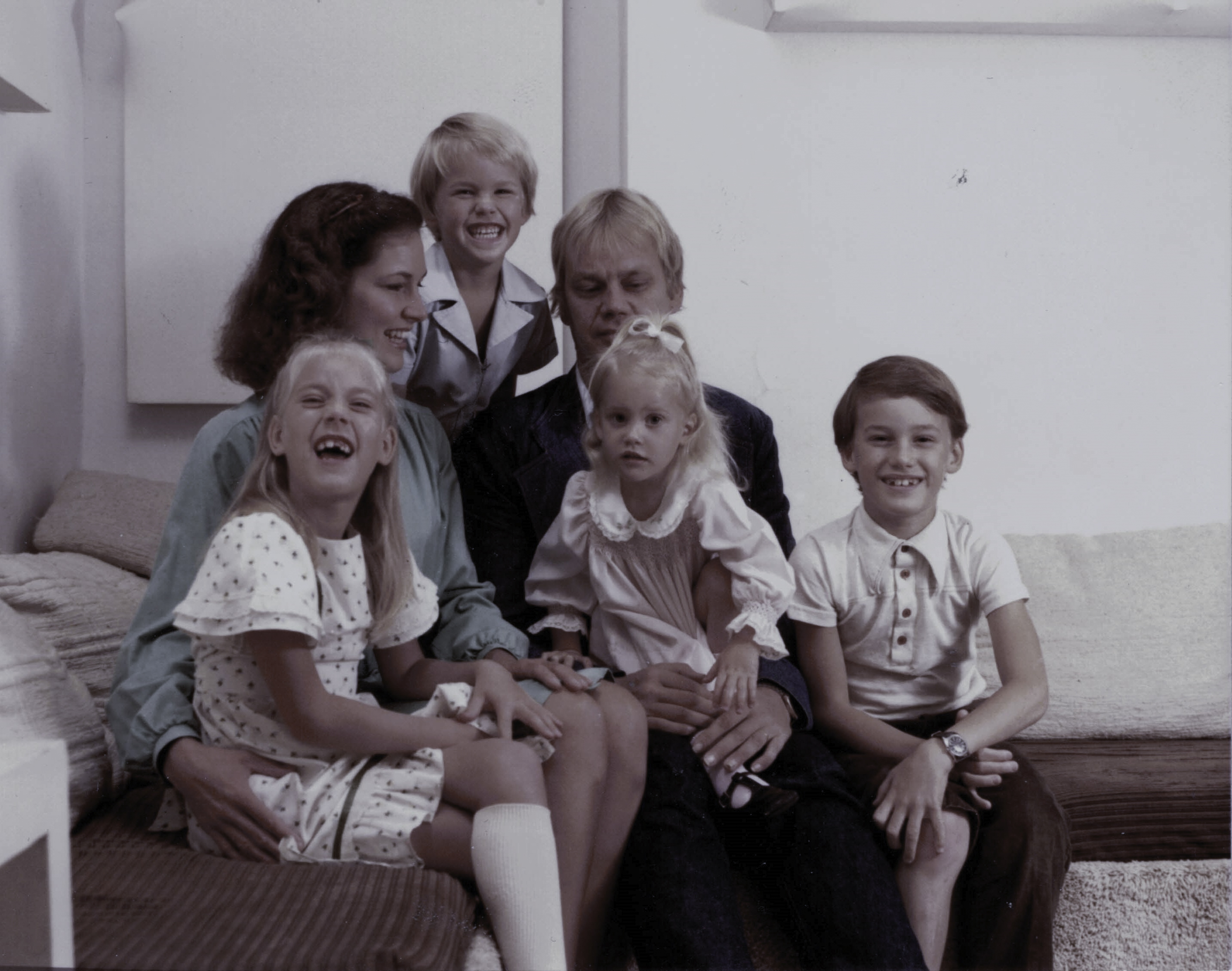
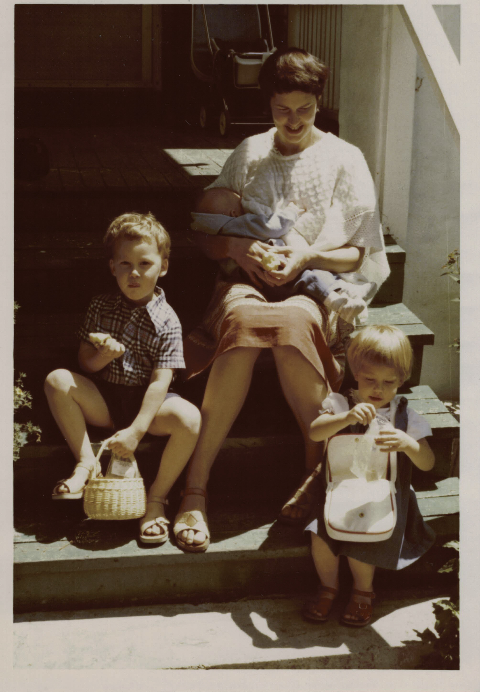
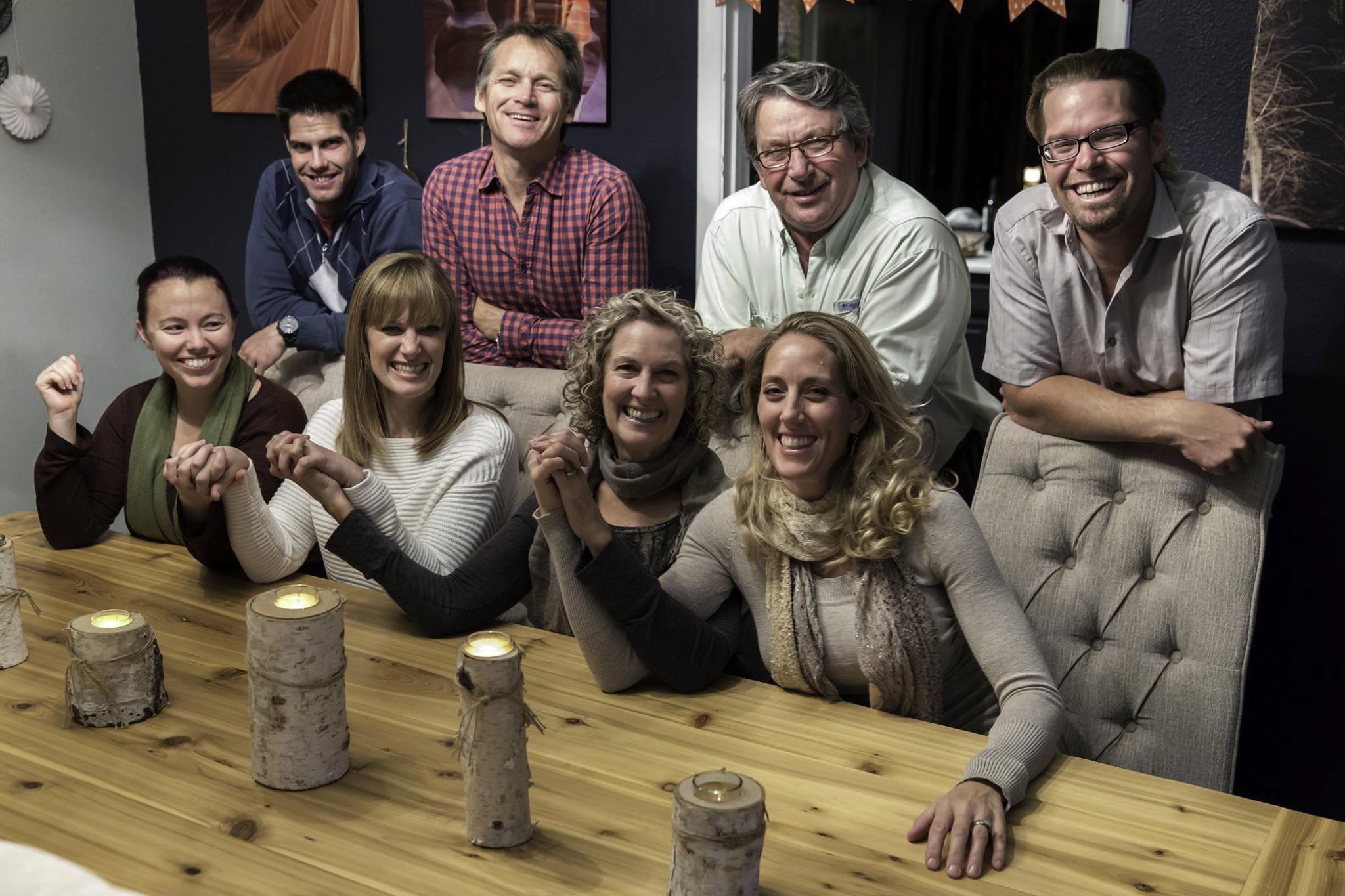
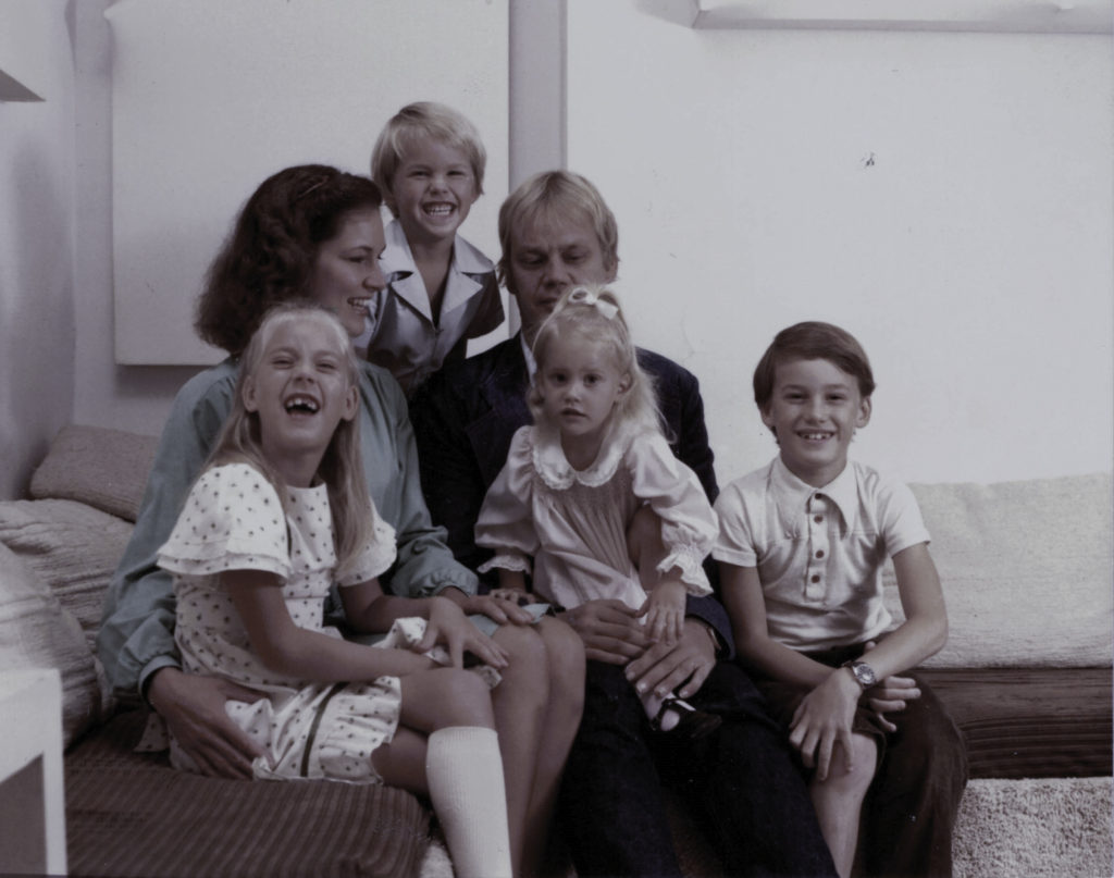
Mom had five kids, myself, Krista, Erik, Karin, and Devin. We grew up fairly poor, not just compared to kids in “the beaches” (with their double lawyer/doctor families), but the household income was low enough that we would have qualified for welfare and other social assistance. Mom wasn’t about to stoop to the level of accepting any such assistance. She worked so hard, that I don’t think we kids really thought of ourselves as poor.
Money was tight enough that very little food was ever wasted, even in extreme situations. There was once a time that mom had scrounged enough to treat us to a home-made cake. We didn’t have air conditioning in that rented house, so the cake (left to cool on the kitchen table before it could be iced) was accessible to anybody that happened to be able to walk in the open front or back doors. A happy little family of racoons invited themselves in that day and sat themselves at the kitchen table to eat the cake that had been left there for them so nicely. Mom walked in on the dining party and screamed. This wasn’t the scream of somebody finding these little beasts in the house, but of having the cake (which she had worked hard to provide and to make) violated – it was supposed to have been a treat for her kids. Within seconds we all rushed to see what was going on and things degenerated into a chaotic Benny Hill like scene, with a human family chasing a family of racoons in circles on the main floor, through the kitchen, living room, dining room and back into the kitchen, and eventually out the doors. Mom tried to salvage the remains of the cake, pleading with us to eat it, exclaiming that “It’s still good!”
Mom, who was a Scientologist, was a model of the Scientology “make it go right” attitude, and we learned that attitude by example. She may have had a shoestring budget, but she was able to see to all our basic requirements, clothes and housing, and of course healthy food. If that meant working a day job, performing late into each night in those smoky piano bars, carrying 3 mortgages, and self-financing her “Checking out of Lonely” album, then so be it. She didn’t let anything get in the way of what needed to be done, and we grew up with her demonstrating, by example, that we could do anything that we set our minds to.
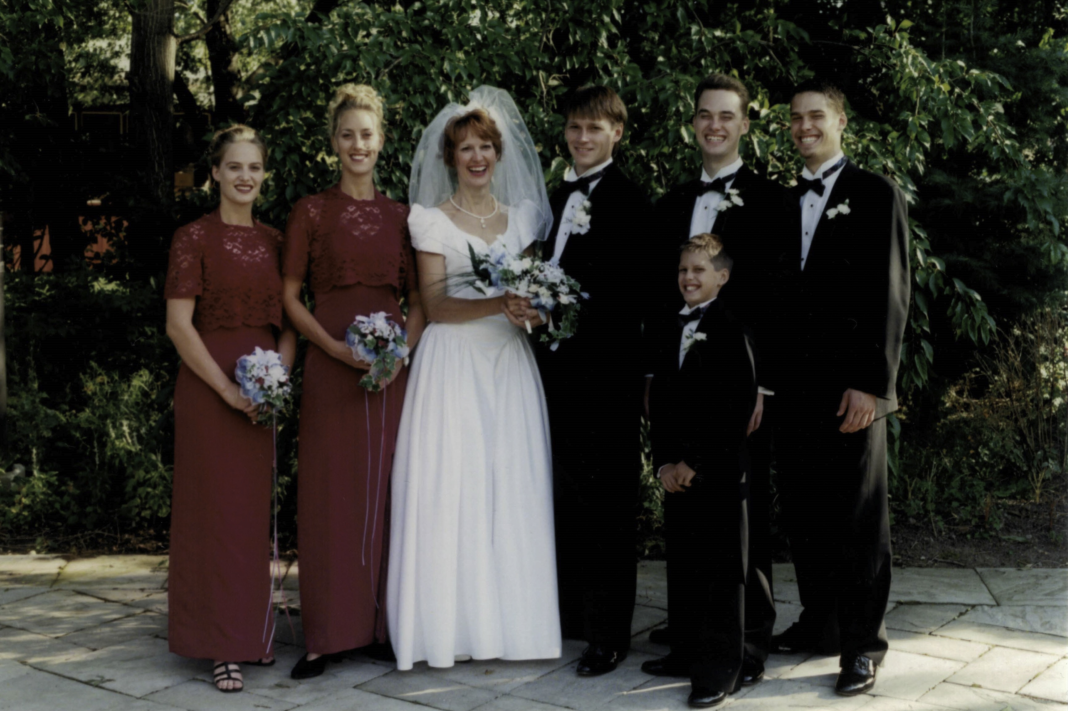
Mom was really proud of all of us. Whatever we happened to be doing, mom raved to everybody about it. She insisted that her kids and grandkids were the best artists, students, photographers, athletes, gymnasts, musicians, and performers. Roles that I got to play for mom included artisan, artist, father of grandkids, engineer, and author. As an author, it happens that my total book sales number 37 (a third of that to family), but a mere fact like that would not dissuade her from a belief that I was her brilliant published author. As kids I think that we all knew that Mom didn’t have an objective opinion of us, and that we weren’t brilliant because “our mom said so”. Despite that, her absolute confidence in our abilities and our capabilities made a big difference in our lives. Like her “make it go right” attitude, we were encouraged to follow our desires and goals where ever they led us. I don’t think that many kids are given such unrestricted opportunities for self-direction, and we were really lucky to have had Mom as a role model, guide and mentor.
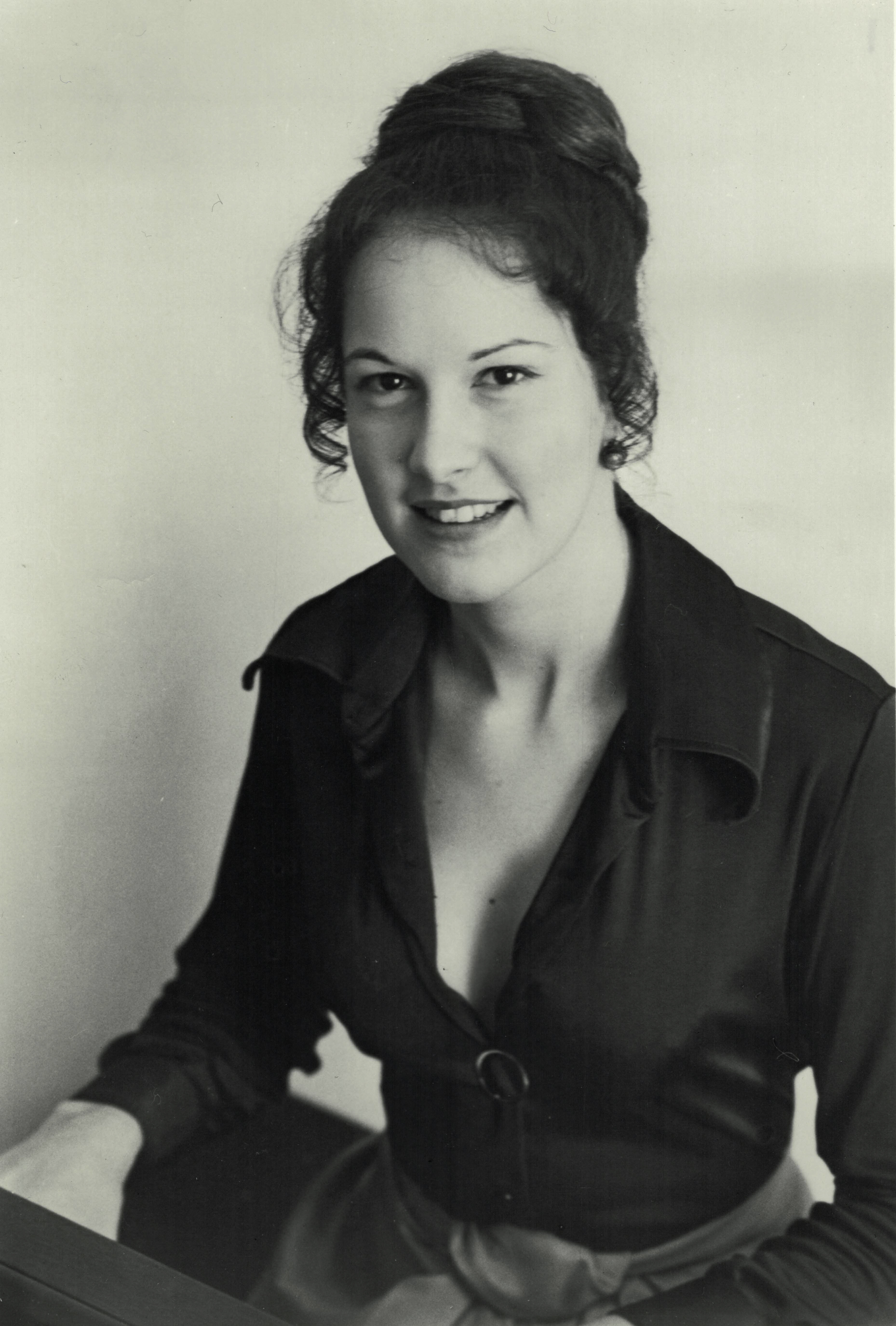
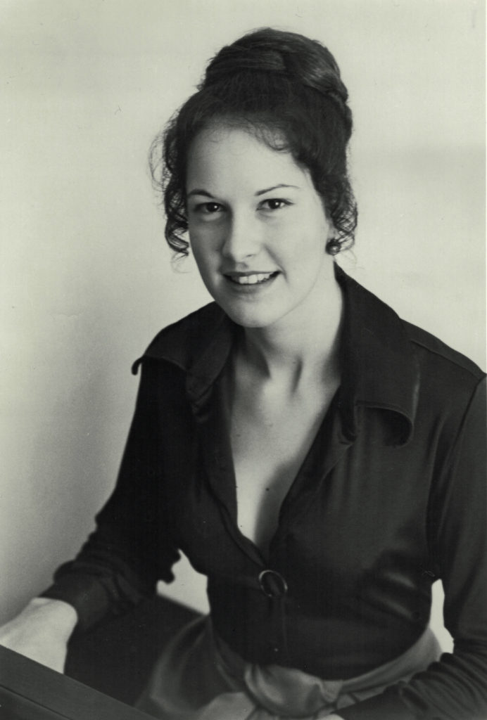
Mom was incredibly smart and talented. I think it would be fair to describe her as a musical prodigy, and she could play intricate piano pieces at a very young age. I’m not sure how many instruments she could play, but they included piano, guitar, voice and even accordion. She could hear just a couple song fragments, and then be able to play them. Her music note books mostly contain only the lyrics to songs, and perhaps a chord annotation or two, since (to her) there was no point writing down anything more. She could even listen to music from memory as if she was hearing it played. Music was an integral part of mom’s life. You couldn’t put music on in the background, since its mere existence required that she stop and listen. That intensity translated to an ability to touch and move people through music that was phenomenal.
I remember mom telling me about a time when she was a kid and snuck some time at the piano to furiously and vigorously play a Beethoven piece. It was a piece which she wasn’t allowed to play, because it wasn’t ladylike to do play that kind of music. Granddad almost caught her, and while she looked at him very guiltily, he told her gently “it’s okay Helen, you can play my Beethoven record.” I’ve wondered what a very young mom would have looked like, pounding the piano, playing that forbidden music? Granddad moved for work a number of times, which provided Mom with opportunities to skip grades a number of times. I think that she said she started college around 16, and she finished so young that her parents still had legal custody of her. After college, she found a composer that she found inspirational, and was able to talk her parents into letting her go to Canada to do a master’s in composition at the University of Toronto.
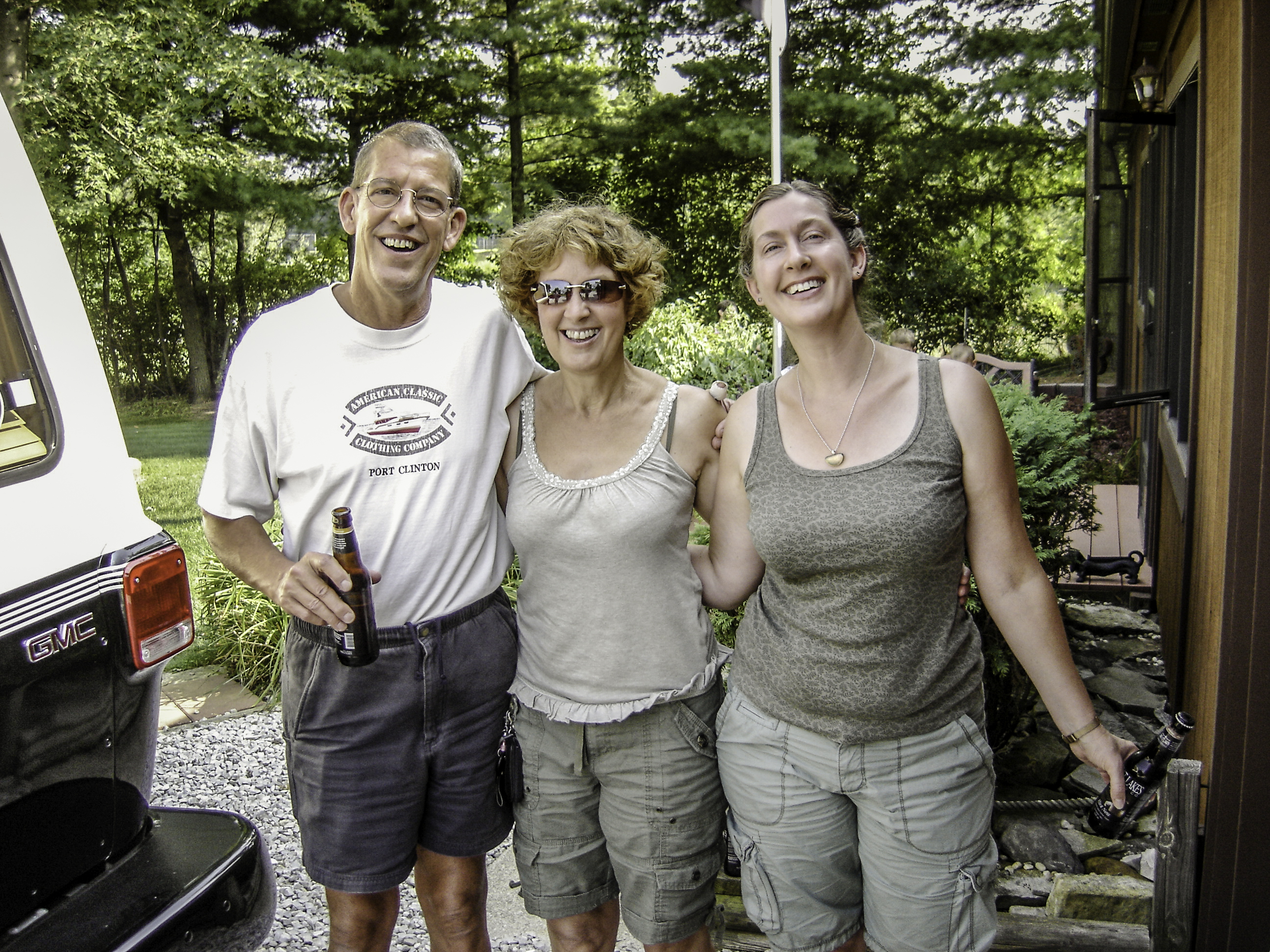
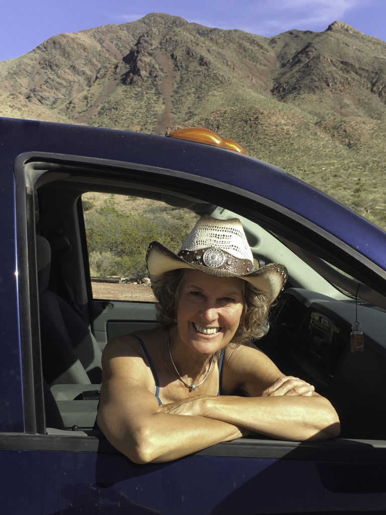
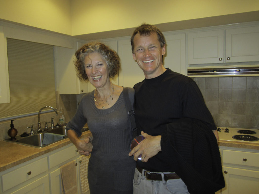
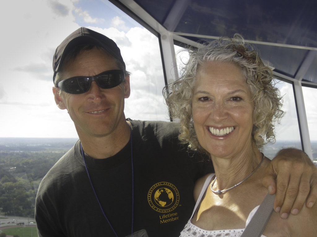
In Toronto Mom met dad, had all of us, transitioned to single-motherhood, and eventually met and married Wade, who I would describe as her soul-mate. Mom and Wade shared a too brief 20+ year life together, touring the United States as together as a dynamic duo delivering “The Wade Henry Show”. Mom’s musical performances tapered off in this time or her life, but despite that, she still continued to inspire and spread joy in all the relationships she formed around the country. If you were to color the path of Mom and Wade around the USA on a map, it would look as if some kids had scribbled all over it!
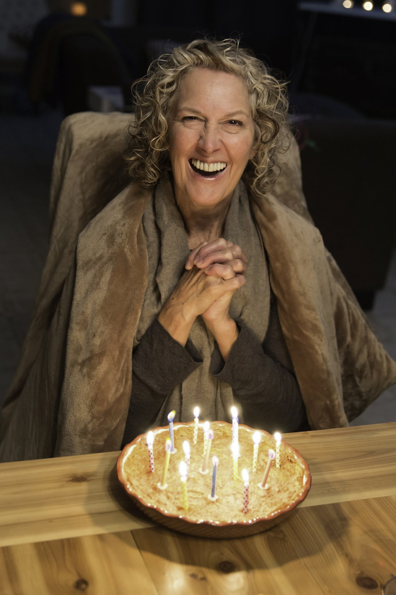
Mom built relationships all over the scribbled path of her life, and she touched the hearts of countless people as she went. Mom, I don’t have good words to describe how much I’ll miss you, and I wonder where you will end up next. I hope that you end up with a nice sturdy set of hiking boots for the next steps of your adventure, where ever that may take you.
Like this:
Like Loading...