This blog now has a copy of all my Mathematica notebooks (as of Feb 10, 2019), complete with a chronological index. I hadn’t updated that index since 2014, and it was quite stale.
I’ve also added an additional level of per-directory indexing. For example, you can now look at just the notebooks for my book, Geometric Algebra for Electrical Engineers. That was possible before, but you would have had to clone the entire git repository to be able to do so easily.
This update includes a new notebook written today, which has a Manipulate visualization of 3D bivector addition that is kind of fun.
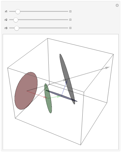
Bivector addition, at least in 3D, can be done graphically almost like vector addition. Instead of trying to add the planes (which can be done, as in the neat illustration in Geometric Algebra for Computer Science), you can do the task more simply by connecting the normals head to tail, where each of the normals are scaled by the area of the bivector (i.e. it’s absolute magnitude). The resulting bivector has an area equal to the length of that sum of normals, and a “direction” perpendicular to that resulting normal. This fun little Manipulate lets you interactively visualize this process, by changing the radius of a set of summed bivectors, each oriented in a different direction, and observing the effects of doing so.
Of course, you can interpret this visualization as nothing more than a representation of addition of cross products, if you were to interpret the vector representing a cross product as an oriented area with a normal equal to that cross product (where the normal’s magnitude equals the area, as in this bivector addition visualization.) This works out nicely because of the duality relationship between the cross and wedge product, and the duality relationship between 3D bivectors and their normals.
Like this:
Like Loading...