[Click here for a PDF of this post with nicer formatting]
Disclaimer
Peeter’s lecture notes from class. These may be incoherent and rough.
Nonlinear systems
On slides, some examples to motivate:
- struts
- fluids
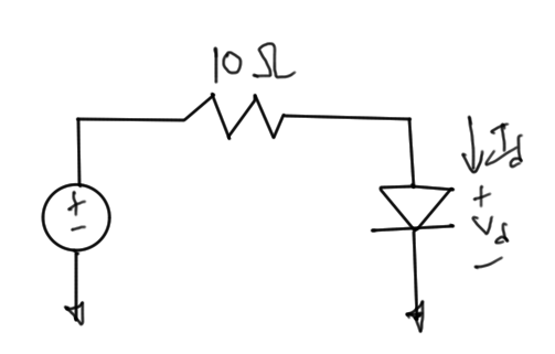
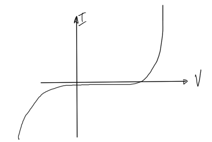
- diode (exponential)Example in fig. 1.
\begin{equation}\label{eqn:multiphysicsL10:20}
I_d = I_s \lr{ e^{V_d/V_t} – 1 } = \frac{10 – V_d}{10}.
\end{equation}
Richardson and Linear Convergence
Seeking the exact solution \( x^\conj \) for
\begin{equation}\label{eqn:multiphysicsL10:40}
f(x^\conj) = 0,
\end{equation}
Suppose that
\begin{equation}\label{eqn:multiphysicsL10:60}
x^{k + 1} = x^k + f(x^k)
\end{equation}
If \( f(x^k) = 0 \) then we have convergence, so \( x^k = x^\conj \).
Convergence analysis
Write the iteration equations at a sample point and the solution as
\begin{equation}\label{eqn:multiphysicsL10:80}
x^{k + 1} = x^k + f(x^k)
\end{equation}
\begin{equation}\label{eqn:multiphysicsL10:100}
x^{\conj} = x^\conj +
\underbrace{
f(x^\conj)
}_{=0}
\end{equation}
Taking the difference we have
\begin{equation}\label{eqn:multiphysicsL10:120}
x^{k+1} – x^\conj = x^k – x^\conj + \lr{ f(x^k) – f(x^\conj) }.
\end{equation}
The last term can be quantified using the mean value theorem \ref{thm:multiphysicsL10:140}, giving
\begin{equation}\label{eqn:multiphysicsL10:140}
x^{k+1} – x^\conj
= x^k – x^\conj +
\evalbar{\PD{x}{f}}{\tilde{x}} \lr{ x^k – x^\conj }
=
\lr{ x^k – x^\conj }
\lr{
1 + \evalbar{\PD{x}{f}}{\tilde{x}} }.
\end{equation}
The absolute value is thus
\begin{equation}\label{eqn:multiphysicsL10:160}
\Abs{x^{k+1} – x^\conj } =
\Abs{ x^k – x^\conj }
\Abs{
1 + \evalbar{\PD{x}{f}}{\tilde{x}} }.
\end{equation}
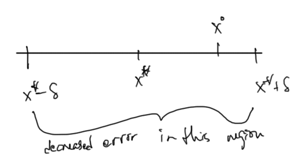
We have convergence provided \( \Abs{ 1 + \evalbar{\PD{x}{f}}{\tilde{x}} } < 1 \) in the region where we happen to iterate over. This could easily be highly dependent on the initial guess.
Stated more accurately we have convergence provided
\begin{equation}\label{eqn:multiphysicsL10:180}
\Abs{
1 + \PD{x}{f} }
\le \gamma < 1
\qquad \forall \tilde{x} \in [ x^\conj – \delta, x^\conj + \delta ],
\end{equation}
and \( \Abs{x^0 – x^\conj } < \delta \). This is illustrated in fig. 3.
It could very easily be difficult to determine the convergence regions.
We have some problems
- Convergence is only linear
- \( x, f(x) \) are not in the same units (and potentially of different orders). For example, \(x\) could be a voltage and \( f(x) \) could be a circuit current.
- (more on slides)
Examples where we may want to use this:
- Spice Gummal Poon transistor model. Lots of diodes, …
- Mosfet model (30 page spec, lots of parameters).
Newton’s method
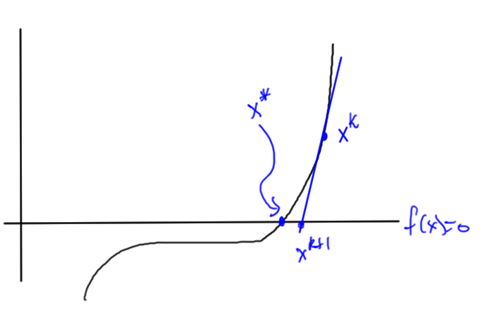
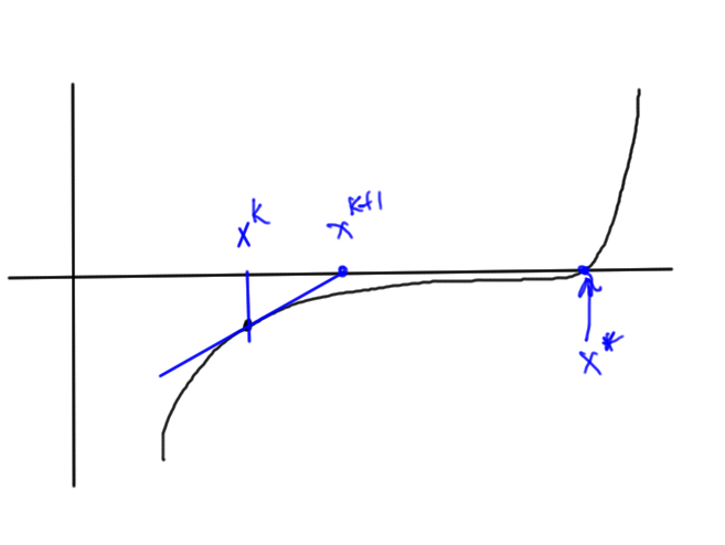
The core idea of this method is sketched in fig. 4. To find the intersection with the x-axis, we follow the slope closer to the intersection.
To do this, we expand \( f(x) \) in Taylor series to first order around \( x^k \), and then solve for \( f(x) = 0 \) in that approximation
\begin{equation}\label{eqn:multiphysicsL10:200}
f( x^{k+1} ) \approx f( x^k ) + \evalbar{ \PD{x}{f} }{x^k} \lr{ x^{k+1} – x^k } = 0.
\end{equation}
This gives
\begin{equation}\label{eqn:multiphysicsL10:220}
\boxed{x^{k+1} = x^k – \frac{f( x^k )}{\evalbar{ \PD{x}{f} }{x^k}}}
\end{equation}
Example: Newton’s method
For the solution of
\begin{equation}\label{eqn:multiphysicsL10:260}
f(x) = x^3 – 2,
\end{equation}
it was found (table 1.1)
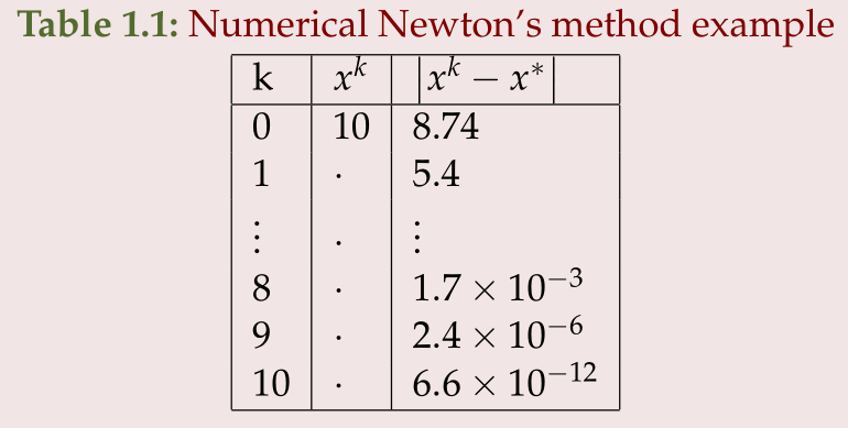
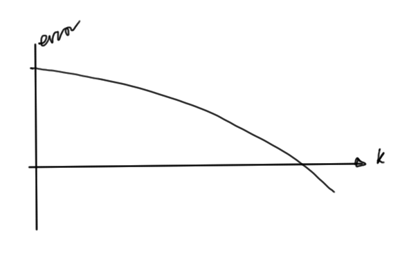
The error tails off fast as illustrated roughly in fig. 6.
Convergence analysis
The convergence condition is
\begin{equation}\label{eqn:multiphysicsL10:280}
0 = f(x^k) + \evalbar{ \PD{x}{f} }{x^k} \lr{ x^{k+1} – x^k }.
\end{equation}
The Taylor series for \( f \) around \( x^k \), using a mean value formulation is
\begin{equation}\label{eqn:multiphysicsL10:300}
f(x)
= f(x^k)
+ \evalbar{ \PD{x}{f} }{x^k} \lr{ x – x^k }.
+ \inv{2} \evalbar{ \PDSq{x}{f} }{\tilde{x} \in [x^\conj, x^k]} \lr{ x – x^k }^2.
\end{equation}
Evaluating at \( x^\conj \) we have
\begin{equation}\label{eqn:multiphysicsL10:320}
0 = f(x^k)
+ \evalbar{ \PD{x}{f} }{x^k} \lr{ x^\conj – x^k }.
+ \inv{2} \evalbar{ \PDSq{x}{f} }{\tilde{x} \in [x^\conj, x^k]} \lr{ x^\conj – x^k }^2.
\end{equation}
and subtracting this from \ref{eqn:multiphysicsL10:280} we are left with
\begin{equation}\label{eqn:multiphysicsL10:340}
0 = \evalbar{\PD{x}{f}}{x^k} \lr{ x^{k+1} – x^k – x^\conj + x^k }
– \inv{2} \evalbar{\PDSq{x}{f}}{\tilde{x}} \lr{ x^\conj – x^k }^2.
\end{equation}
Solving for the difference from the solution, the error is
\begin{equation}\label{eqn:multiphysicsL10:360}
x^{k+1} – x^\conj
= \inv{2} \lr{ \PD{x}{f} }^{-1} \evalbar{\PDSq{x}{f}}{\tilde{x}} \lr{ x^k – x^\conj }^2,
\end{equation}
or in absolute value
\begin{equation}\label{eqn:multiphysicsL10:380}
\Abs{ x^{k+1} – x^\conj }
= \inv{2} \Abs{ \PD{x}{f} }^{-1} \Abs{ \PDSq{x}{f} } \Abs{ x^k – x^\conj }^2.
\end{equation}
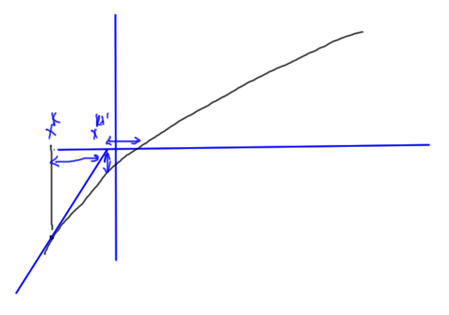
We see that convergence is quadratic in the error from the previous iteration. We will have trouble if the derivative goes small at any point in the iteration region, for example in fig. 7, we could easily end up in the zero derivative region.
When to stop iteration
One way to check is to look to see if the difference
\begin{equation}\label{eqn:multiphysicsL10:420}
\Norm{ x^{k+1} – x^k } < \epsilon_{\Delta x},
\end{equation}
however, when the function has a very step slope
this may not be sufficient unless we also substitute our trial solution and see if we have the match desired.
Alternatively, if the slope is shallow as in fig. 7, then checking for just \( \Abs{ f(x^{k+1} } < \epsilon_f \) may also mean we are off target.
Finally, we may also need a relative error check to avoid false convergence. In fig. 10, we may have both
\begin{equation}\label{eqn:multiphysicsL10:440}
\Abs{x^{k+1} – x^k} < \epsilon_{\Delta x}
\end{equation}
\begin{equation}\label{eqn:multiphysicsL10:460}
\Abs{f(x^{k+1}) } < \epsilon_{f},
\end{equation}
however, we may also want a small relative difference
\begin{equation}\label{eqn:multiphysicsL10:480}
\frac{\Abs{x^{k+1} – x^k}}{\Abs{x^k}}
< \epsilon_{f,r}.
\end{equation}
This can become problematic in real world engineering examples such as to diode of fig. 11, where we have shallow regions and fast growing or dropping regions.
Theorems
Mean value theorem
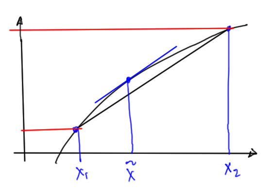
For a continuous and differentiable function \( f(x) \), the difference can be expressed in terms of the derivative at an intermediate point
\begin{equation*}
f(x_2) – f(x_1)
= \evalbar{ \PD{x}{f} }{\tilde{x}} \lr{ x_2 – x_1 }
\end{equation*}
where \( \tilde{x} \in [x_1, x_2] \).
This is illustrated (roughly) in fig. 2.
