What’s in the pipe.

It’s been a while since I did any math or physics writing. This is the first post in a series where I plan to work my way systematically from an introduction of vectors, to the axioms of geometric algebra. I plan to start with an introduction of vectors as directed “arrows”, building on that to discuss coordinates, tuples, and column matrix representations, and representation independent ideas. With those basics established, I’ll remind the reader about how generalized vector and dot product spaces are defined and give some examples. Finally, with the foundation of vectors and vector spaces in place, I’ll introduce the concept of a multivector space, and the geometric product, and start unpacking the implications of the axioms that follow naturally from this train of thought.

The applications that I plan to include in this series will be restricted to Euclidean spaces (i.e. where length is given by the Pythagorean law), primarily those of 2 and 3 dimensions. However, it will be good to also lay the foundations for the non-Euclidean spaces that we encounter in relativistic electromagnetism (there is actually no other kind), and in computer graphics applications of geometric algebra, especially since we can do so nearly for free. I plan to try to introduce the requisite ideas (i.e. the metric, which allows for a generalized dot product) by discussing Euclidean non-orthonormal bases. Such bases have applications in condensed matter physics where there are useful for modelling crystal and lattice structure, and provide a hands conceptual bridge to a set of ideas that might otherwise seem abstract and without “real world” application.

Motivation.

Many introductions to geometric algebra start by first introducing the dot product, then bivectors and the wedge product, and eventually define the product of two vectors as the synthetic sum of the dot and wedge
\begin{equation}\label{eqn:multivector:20}
\Bx \By = \Bx \cdot \By + \Bx \wedge \By.
\end{equation}
It takes a fair amount of work to do this well. In the seminal work [4] a few pages are taken for each of the dot and wedge products, showing the similarities and building up ideas, before introducing the geometric product in this fashion. In [2] the authors take a phenomenal five chapters to build up the context required to introduce the geometric product. I am not disparaging the authors for taking that long to build up the ideas, as their introduction of the subject is exceedingly clear and thorough, and they do a lot more than the minumum required to define the geometric product.

The strategy to introduce the geometric product as a sum of dot and wedge can result in considerable confusion, especially since the wedge product is often defined in terms of the geometric product
\begin{equation}\label{eqn:multivector:40}
\Bx \wedge \By =
\inv{2} \lr{
\Bx \By – \By \Bx
}.
\end{equation}
The whole subject can appear like a chicken and egg problem. I personally found the subject very confusing initially, and had considerable difficulty understanding which of the many identities of geometric algebra were the most fundamental. For this reason, I found the axiomatic approach of [1] very refreshing. The cavaet with that work is that is is exceptionally terse, as they jammed a reformulation of most of physics using geometric algebra into that single book, and it would have been thousands of pages had they tried to make it readable by mere mortals.

When I wrote my own book on geometric algebra, I had the intuition that the way to introduce the subject ought to be like the vector space in abstract linear algebra. The construct of a vector space is a curious and indirect way to define a vector. Vectors are not defined as entities, but simply as members of a vector space, a space that is required to have a set of properties. I thought that the same approach would probably work with multivectors, which could be defined as members of a multivector space, a mathematical construction with a set of properties.

I did try this approach, but was not fully satisfied with what I wrote. I think that dissatisfaction was because I tried to define the multivector first. To define the multivector, I first introduced a whole set of prerequisite ideas (bivector, trivector, blade, k-vector, vector product, …), but that was also problematic, since the vector multiplication idea required for those concepts wasn’t fully defined until the multivector space itself was defined.

My approach shows some mathematical cowardness. Had I taken the approach of the vector space fully to heart, the multivector could have been defined as a member of a multivector space, and all the other ideas follow from that. In this multi-part series, I’m going to play with this approach anew, and see how it works out. If it does work, I’ll see if I can incorporate this approach into a new version of my book.

Review and background.

In this series, I’m going to assume a reader interested in geometric algebra, is probably also familiar with a wide variety of concepts, including but not limited to

vectors,
coordinates,
matrices,
basis,
change of basis,
dot product,
real and complex numbers,
rotations and translations,
vector spaces, and
linear transformations.

Despite those assumptions, as mentioned above, I’m going to attempt to build up the basics of vector representation and vector spaces in a systematic fashion, starting from a very elementary level.

My reasons for doing so are mainly to explore the logical sequencing of the ideas required. I’ve always found well crafted pedagogical sequences rewarding, and will hopefully construct one here that is appreciated by anybody who chooses to follow along.

Next time.

As preparation for the next article in this series, the reader is asked to watch a short lesson from Vector, not so supervillain extraordinaire (Despicable Me).

References

[1] C. Doran and A.N. Lasenby. Geometric algebra for physicists. Cambridge University Press New York, Cambridge, UK, 1st edition, 2003.

[2] L. Dorst, D. Fontijne, and S. Mann. Geometric Algebra for Computer Science. Morgan Kaufmann, San Francisco, 2007.

[4] D. Hestenes. New Foundations for Classical Mechanics. Kluwer Academic Publishers, 1999.

[Click here for a PDF of this post with nicer formatting]

Disclaimer

Peeter’s lecture notes from class. These may be incoherent and rough.

These are notes for the UofT course ECE1505H, Convex Optimization, taught by Prof. Stark Draper, from [1].

Topics

Calculus: Derivatives and Jacobians, Gradients, Hessians, approximation functions.
Linear algebra, Matrices, decompositions, …

Norms

Vector space:

A set of elements (vectors) that is closed under vector addition and scaling.

This generalizes the directed arrow concept of vector space (fig. 1) that is familiar from geometry.

fig. 1. Vector addition.

Normed vector spaces:

A vector space with a notion of length of any single vector, the “norm”.

Inner product space:
A normed vector space with a notion of a real angle between any pair of vectors.

This course has a focus on optimization in \R{n}. Complex spaces in the context of this course can be considered with a mapping \( \text{\C{n}} \rightarrow \mathbb{R}^{2 n} \).

Norm:
A norm is a function operating on a vector

\begin{equation*}
\Bx = ( x_1, x_2, \cdots, x_n )
\end{equation*}

that provides a mapping

\begin{equation*}
\Norm{ \cdot } : \mathbb{R}^{n} \rightarrow \mathbb{R},
\end{equation*}

where

\( \Norm{ \Bx } \ge 0 \)
\( \Norm{ \Bx } = 0 \qquad \iff \Bx = 0 \)
\( \Norm{ t \Bx } = \Abs{t} \Norm{ \Bx } \)
\( \Norm{ \Bx + \By } \le \Norm{ \Bx } + \Norm{\By} \). This is the triangle inequality.

Example: Euclidean norm

\begin{equation}\label{eqn:convex-optimizationLecture2:24}
\Norm{\Bx} = \sqrt{ \sum_{i = 1}^n x_i^2 }
\end{equation}

Example: \(l_p\)-norms

\begin{equation}\label{eqn:convex-optimizationLecture2:44}
\Norm{\Bx}_p = \lr{ \sum_{i = 1}^n \Abs{x_i}^p }^{1/p}.
\end{equation}

For \( p = 1 \), this is

\begin{equation}\label{eqn:convex-optimizationLecture2:64}
\Norm{\Bx}_1 = \sum_{i = 1}^n \Abs{x_i},
\end{equation}

For \( p = 2 \), this is the Euclidean norm \ref{eqn:convex-optimizationLecture2:24}.
For \( p = \infty \), this is

\begin{equation}\label{eqn:convex-optimizationLecture2:324}
\Norm{\Bx}_\infty = \max_{i = 1}^n \Abs{x_i}.
\end{equation}

Unit ball:

\begin{equation*}
\setlr{ \Bx | \Norm{\Bx} \le 1 }
\end{equation*}

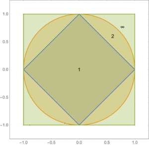
The regions of the unit ball under the \( l_1, l_2, and l_\infty \) norms are plotted in fig. 2.

fig. 2. Some unit ball regions.

The \( l_2 \) norm is not only familiar, but can be “induced” by an inner product

\begin{equation}\label{eqn:convex-optimizationLecture2:84}
\left\langle \Bx, \By \right\rangle = \Bx^\T \By = \sum_{i = 1}^n x_i y_i,
\end{equation}

which is not true for all norms. The norm induced by this inner product is

\begin{equation}\label{eqn:convex-optimizationLecture2:104}
\Norm{\Bx}_2 = \sqrt{ \left\langle \Bx, \By \right\rangle }
\end{equation}

Inner product spaces have a notion of angle (fig. 3) given by

\begin{equation}\label{eqn:convex-optimizationLecture2:124}
\left\langle \Bx, \By \right\rangle = \Norm{\Bx} \Norm{\By} \cos \theta,
\end{equation}

fig. 3. Inner product induced angle.

and always satisfy the Cauchy-Schwartz inequality

\begin{equation}\label{eqn:convex-optimizationLecture2:144}
\left\langle \Bx, \By \right\rangle \le \Norm{\Bx}_2 \Norm{\By}_2.
\end{equation}

In an inner product space we say \( \Bx \) and \( \By \) are orthogonal vectors \( \Bx \perp \By \) if \( \left\langle \Bx, \By \right\rangle = 0 \), as sketched in fig. 4.

fig. 4. Orthogonality.

Dual norm

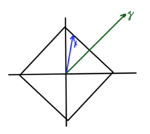
Let \( \Norm{ \cdot } \) be a norm in \R{n}. The “dual” norm \( \Norm{ \cdot }_\conj \) is defined as

\begin{equation*}
\Norm{\Bz}_\conj = \sup_\Bx \setlr{ \Bz^\T \Bx | \Norm{\Bx} \le 1 }.
\end{equation*}

where \( \sup \) is roughly the “least upper bound”.
\index{sup}

This is a limit over the unit ball of \( \Norm{\cdot} \).

\( l_2 \) dual

Dual of the \( l_2 \) is the \( l_2 \) norm.

fig. 5. l_2 dual norm determination.

Proof:

\begin{equation}\label{eqn:convex-optimizationLecture2:164}
\begin{aligned}
\Norm{\Bz}_\conj
&= \sup_\Bx \setlr{ \Bz^\T \Bx | \Norm{\Bx}_2 \le 1 } \\
&= \sup_\Bx \setlr{ \Norm{\Bz}_2 \Norm{\Bx}_2 \cos\theta | \Norm{\Bx}_2 \le 1 } \\
&\le \sup_\Bx \setlr{ \Norm{\Bz}_2 \Norm{\Bx}_2 | \Norm{\Bx}_2 \le 1 } \\
&\le
\Norm{\Bz}_2
\Norm{
\frac{\Bz}{ \Norm{\Bz}_2 }
}_2 \\
&=
\Norm{\Bz}_2.
\end{aligned}
\end{equation}

\( l_1 \) dual

For \( l_1 \), the dual is the \( l_\infty \) norm. Proof:

\begin{equation}\label{eqn:convex-optimizationLecture2:184}
\Norm{\Bz}_\conj
=
\sup_\Bx \setlr{ \Bz^\T \Bx | \Norm{\Bx}_1 \le 1 },
\end{equation}

but
\begin{equation}\label{eqn:convex-optimizationLecture2:204}
\Bz^\T \Bx
=
\sum_{i=1}^n z_i x_i \le
\Abs{
\sum_{i=1}^n z_i x_i
}
\le
\sum_{i=1}^n \Abs{z_i x_i },
\end{equation}

so
\begin{equation}\label{eqn:convex-optimizationLecture2:224}
\begin{aligned}
\Norm{\Bz}_\conj
&=
\sum_{i=1}^n \Abs{z_i}\Abs{ x_i } \\
&\le \lr{ \max_{j=1}^n \Abs{z_j} }
\sum_{i=1}^n \Abs{ x_i } \\
&\le \lr{ \max_{j=1}^n \Abs{z_j} } \\
&=
\Norm{\Bz}_\infty.
\end{aligned}
\end{equation}

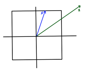
\( l_\infty \) dual

fig. 6. l_1 dual norm determination.

fig. 7. l_\infinity dual norm determination.

\begin{equation}\label{eqn:convex-optimizationLecture2:244}
\Norm{\Bz}_\conj
=
\sup_\Bx \setlr{ \Bz^\T \Bx | \Norm{\Bx}_\infty \le 1 }.
\end{equation}

Here
\begin{equation}\label{eqn:convex-optimizationLecture2:264}
\begin{aligned}
\Bz^\T \Bx
&=
\sum_{i=1}^n z_i x_i \\
&\le
\sum_{i=1}^n \Abs{z_i}\Abs{ x_i } \\
&\le
\lr{ \max_j \Abs{ x_j } }
\sum_{i=1}^n \Abs{z_i} \\
&=
\Norm{\Bx}_\infty
\sum_{i=1}^n \Abs{z_i}.
\end{aligned}
\end{equation}

So
\begin{equation}\label{eqn:convex-optimizationLecture2:284}
\Norm{\Bz}_\conj
\le
\sum_{i=1}^n \Abs{z_i}
=
\Norm{\Bz}_1.
\end{equation}

Statement from the lecture: I’m not sure where this fits:

\begin{equation}\label{eqn:convex-optimizationLecture2:304}
x_i^\conj
=
\left\{
\begin{array}{l l}
+1 & \quad \mbox{\( z_i \ge 0 \)} \\
-1 & \quad \mbox{\( z_i \le 0 \)}
\end{array}
\right.
\end{equation}

References

[1] Stephen Boyd and Lieven Vandenberghe. Convex optimization. Cambridge university press, 2004.

vector space

[Series intro] An introduction to geometric algebra.

What’s in the pipe.

Motivation.

Review and background.

Next time.

References

Like this: