wolfram CDF

Chebychev antenna array design

March 22, 2015 ece1229 , , , ,

[Click here for a PDF of this post with nicer formatting]

In our text [1] is a design procedure that applies Chebychev polynomials to the selection of current magnitudes for an evenly spaced array of identical antennas placed along the z-axis.

For an even number \( 2 M \) of identical antennas placed at positions \( \Br_m = (d/2) \lr{2 m -1} \Be_3 \), the array factor is

\begin{equation}\label{eqn:chebychevDesign:20}
\textrm{AF}
=
\sum_{m=-N}^N I_m e^{-j k \rcap \cdot \Br_m }.
\end{equation}

Assuming the currents are symmetric \( I_{-m} = I_m \), with \( \rcap = (\sin\theta \cos\phi, \sin\theta \sin\phi, \cos\theta ) \), and \( u = \frac{\pi d}{\lambda} \cos\theta \), this is

\begin{equation}\label{eqn:chebychevDesign:40}
\begin{aligned}
\textrm{AF}
&=
\sum_{m=-N}^N I_m e^{-j k (d/2) ( 2 m -1 )\cos\theta } \\
&=
2 \sum_{m=1}^N I_m \cos\lr{ k (d/2) ( 2 m -1)\cos\theta } \\
&=
2 \sum_{m=1}^N I_m \cos\lr{ (2 m -1) u }.
\end{aligned}
\end{equation}

This is a sum of only odd cosines, and can be expanded as a sum that includes all the odd powers of \( \cos u \). Suppose for example that this is a four element array with \( N = 2 \). In this case the array factor has the form

\begin{equation}\label{eqn:chebychevDesign:60}
\begin{aligned}
\textrm{AF}
&=
2 \lr{ I_1 \cos u + I_2 \lr{ 4 \cos^3 u – 3 \cos u } } \\
&=
2 \lr{ \lr{ I_1 – 3 I_2 } \cos u + 4 I_2 \cos^3 u }.
\end{aligned}
\end{equation}

The design procedure in the text sets \( \cos u = z/z_0 \), and then equates this to \( T_3(z) = 4 z^3 – 3 z \) to determine the current amplitudes \( I_m \). That is

\begin{equation}\label{eqn:chebychevDesign:80}
\frac{ 2 I_1 – 6 I_2 }{z_0} z + \frac{8 I_2}{z_0^3} z^3 = -3 z + 4 z^3,
\end{equation}

or

\begin{equation}\label{eqn:chebychevDesign:100}
\begin{aligned}
\begin{bmatrix}
I_1 \\
I_2
\end{bmatrix}
&=
{\begin{bmatrix}
2/z_0 & -6/z_0 \\
0 & 8/z_0^3
\end{bmatrix}}^{-1}
\begin{bmatrix}
-3 \\
4
\end{bmatrix} \\
&=
\frac{z_0}{2}
\begin{bmatrix}
3 (z_0^2 -1) \\
z_0^2
\end{bmatrix}.
\end{aligned}
\end{equation}

The currents in the array factor are fully determined up to a scale factor, reducing the array factor to

\begin{equation}\label{eqn:chebychevDesign:140}
\textrm{AF} = 4 z_0^3 \cos^3 u – 3 z_0 \cos u.
\end{equation}

The zeros of this array factor are located at the zeros of

\begin{equation}\label{eqn:chebychevDesign:120}
T_3( z_0 \cos u ) = \cos( 3 \cos^{-1} \lr{ z_0 \cos u } ),
\end{equation}

which are at \( 3 \cos^{-1} \lr{ z_0 \cos u } = \pi/2 + m \pi = \pi \lr{ m + \inv{2} } \)

\begin{equation}\label{eqn:chebychevDesign:160}
\cos u = \inv{z_0} \cos\lr{ \frac{\pi}{3} \lr{ m + \inv{2} } } = \setlr{ 0, \pm \frac{\sqrt{3}}{2 z_0} }.
\end{equation}

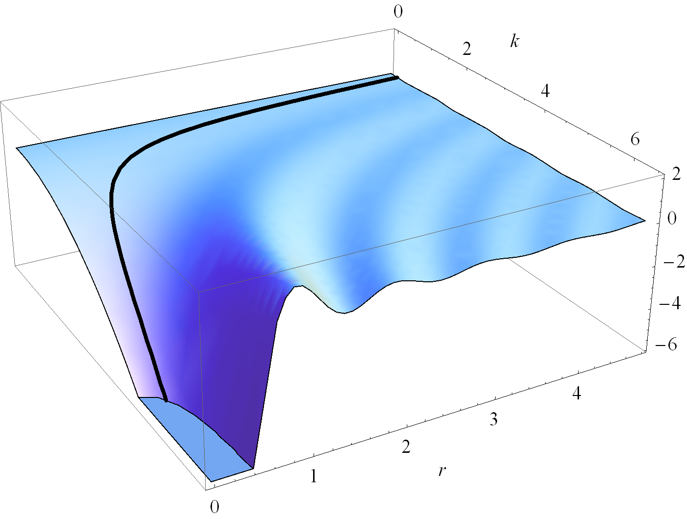
showing that the scaling factor \( z_0 \) effects the locations of the zeros. It also allows the values at the extremes \( \cos u = \pm 1 \), to increase past the \( \pm 1 \) non-scaled limit values. These effects can be explored in this Mathematica notebook, but can also be seen in fig. 1.

ChebyChevThreeScaledFig2pn

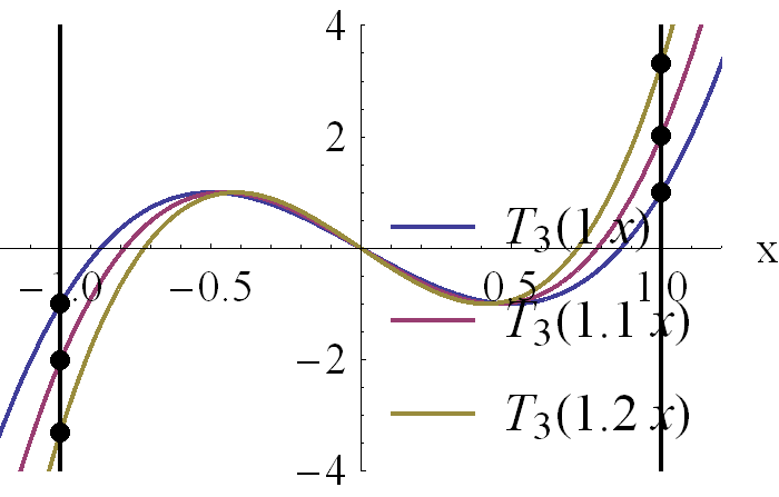
fig 1. T_3( z_0 x) for a few different scale factors z_0.


The scale factor can be fixed for a desired maximum power gain. For \( R
\textrm{dB} \), that will be when

\begin{equation}\label{eqn:chebychevDesign:180}
20 \log_{10} \cosh( 3 \cosh^{-1} z_0 ) = R \textrm{dB},
\end{equation}

or

\begin{equation}\label{eqn:chebychevDesign:200}
z_0 = \cosh \lr{ \inv{3} \cosh^{-1} \lr{ 10^{\frac{R}{20}} } }.
\end{equation}

For \( R = 30 \) dB (say), we have \( z_0 = 2.1 \), and

\begin{equation}\label{eqn:chebychevDesign:220}
\textrm{AF}
= 40 \cos^3 \lr{ \frac{\pi d}{\lambda} \cos\theta } – 6.4 \cos \lr{ \frac{\pi d}{\lambda} \cos\theta }.
\end{equation}

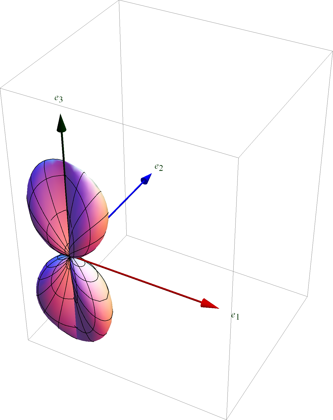
These are plotted in fig. 2 (linear scale), and fig. 3 (dB scale) for a couple values of \( d/\lambda \).

ChebychevT3FittingFig3pn

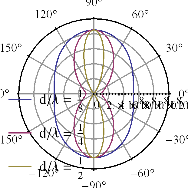
fig 2. T_3 fitting of 4 element array (linear scale).

ChebychevT3FittingDbFig4pn

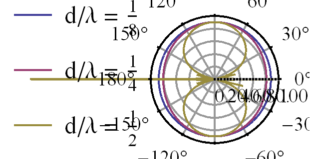
fig 3. T_3 fitting of 4 element array (dB scale).

To explore the \( d/\lambda \) dependence try this Mathematica notebook.

References

[1] Constantine A Balanis. Antenna theory: analysis and design. John
Wiley & Sons, 3rd edition, 2005.

Mathematica CDF notebooks for ece1229 (antenna theory)

February 8, 2015 ece1229 , ,

TaiAndPereiraSampleFieldThetaCapComponentFig1pn

infinitesimalDipoleErRealFig1pn

I put together a couple of cool Manipulate notebooks for some radiation plots.

I am not able to share these directly as blog posts since the CDF plugin that I am using in my wordpress instance appears to have a new plugin or version incompatibility, and is no longer working. The link above has some plain html javascript wrappers for these notebooks, and works at least with chrome and firefox on windows 7.

Pick a number between 1 and 10

July 14, 2014 math and physics play , , , ,

I saw the following on mathfail.com (EDIT: dead link), and thought about it a bit


Notice that the +4 here is entirely misdirection.  This is really just a statement that the sum of the digits of any integer power of 9 up to 81, is 9.

It also appears to be true that, for integer a in \([1, N+1]\)

\[(N a) \text{div} (N+1) + (N a) \text{mod} (N + 1) = N.\]

This is demonstrated in the following Mathematica Manipulate

However, I’m unsure how to prove or disprove this?

How much difference will shopping around for mortgage rates make?

June 17, 2014 Incoherent ramblings , , , , , , , ,

[Click here for a standalone PDF of this post]

Motivation

The banks are all offering variable rate mortgages at slight differences from prime (current 3%). I have asked for a few competing rate quotes to see which is best.

Scotiabank offered \(\text{prime} – 0.53\%\). PC Financial offered \(\text{prime} – 0.55\%\), slightly better. ING’s offer wasn’t competitive at \(\text{prime} – 0.25\%\). BMO offered the best so far at \(\text{prime} – 0.6\%\), with the conditions that we’d have to open joint chequing and a joint BMO mastercard. Royal’s default offering matched PC Financial’s offer at \(\text{prime} – 0.55\%\), and she’s now playing the back room manager game to see if she can get approval to beat (or even match) BMO’s offer.

Let’s compare those here and see how much difference these quotes result in. Is it even worth it to do this negotiation?

Guts

Consider first a principle amount \(-P\), and set of payments \(A, B, C, D, …\), equally spaced in time, corresponding with some effective interest rate per period. This is sketched in fig 1.1.

Fig 1.1: Payments at fixed intervals

Fig 1.1: Payments at fixed intervals


We want to refresh our memory about future value calculations for such a set of payments. Suppose the interest rate per period is \(i\), for example \(i = 0.03\) for a 3% rate, then at the first, second, third, and fourth intervals, we have respectively

\begin{equation}\label{eqn:mortgageInterest:20}
\begin{aligned}
-P(1 + i) + A & \\
\lr{ -P(1 + i) + A }(1 + i) + B &= -P(1+i)^2 + A(1 + i) + B \\
\lr{ \lr{ -P(1 + i) + A }(1 + i) + B}(1 + i) + C &= -P(1+i)^3 + A(1 + i)^2 + B(1 + i) + C \\
\lr{ \lr{ \lr{ -P(1 + i) + A }(1 + i) + B}(1 + i) + C}(1 + i) + D
&= -P(1+i)^4 + A(1 + i)^3 + B(1 + i)^2 + C(1+i) + D.
\end{aligned}
\end{equation}

We can treat the payments independently, each with a separate \((1+i)^k\) factor adjusting the future value of that payment. The case where the payments are of equal value is of particular interest. For that, after \(k\) payments, the future value of the initial principle offset by any of the payments is

\begin{equation}\label{eqn:mortgageInterest:40}
F_k
= -P(1+i)^k + A(1 + i)^{k-1} + A(1 + i)^{k-2} + \cdots A.
\end{equation}

Recall that a geometric sum

\begin{equation}\label{eqn:mortgageInterest:60}
S_k = 1 + a + a^2 + \cdots + a^{k-1},
\end{equation}

can be solved by writing

\begin{equation}\label{eqn:mortgageInterest:80}
a S_k – S_k = a^k – 1,
\end{equation}

so that

\begin{equation}\label{eqn:mortgageInterest:100}
S_k = \frac{a^k – 1}{a – 1}.
\end{equation}

The future value thus sums to

\begin{equation}\label{eqn:mortgageInterest:120}
F_k
=
-P(1+i)^k + A \frac{ (1 + i)^k – 1}{ 1 + i – 1 },
\end{equation}

or
\begin{equation}\label{eqn:mortgageInterest:160}
\boxed{
F_k
=
\lr{ -P + \frac{A}{i} } (1 + i)^k – \frac{A}{i}.
}
\end{equation}

Observe that we can invert \ref{eqn:mortgageInterest:160} for \(k\) by taking logs of the inequality \(F_k \ge 0\). This gives

\begin{equation}\label{eqn:mortgageInterest:180}
\boxed{
k \ge – \frac{\ln\lr{ 1 – i P/A}}{\ln\lr{1 + i}}
}
\end{equation}

It’s clear that we are in trouble (with always negative future value, and no solution to the inequality) unless \(-P + A/i > 0\), or

\begin{equation}\label{eqn:mortgageInterest:140}
A > i P.
\end{equation}

For example, at \(i = 3\%\) interest per year, compounded monthly, the monthly break even payment rate for various mortgage amounts \(P\) is tabulated in table 1.1

This provides a first hint that the 0.5-0.6 less than prime rates that the various banks offer will make a difference. For a principle of \(200 K\), we require \(17\) dollars more per month to break even (not paying down the principle at all) when comparing prime less \(0.5\%\) and \(0.6\%\).

Suppose we make \(1000\) per month payments at prime minus various amounts. At the end of a 5 year (60 month) term, we have the following future values

With a mortgage amount of 225K and the nominal monthly payment amount of 1K, is this negotiation worth the time? It appears that finding somebody willing to loan at prime minus 0.6% vs. prime minus 0.5% is only worth about $550 after five years. That saving amounts to about 1.5 months of the banks interest profit.

It’s interesting to see that, despite the bank making on the order of 25K for such a mortgage after five years, how little they are willing to move in their adjustment of interest rates.

If you have the wolfram CDF plugin installed, equations \ref{eqn:mortgageInterest:120}, and \ref{eqn:mortgageInterest:160} can be executed using the following simple monthly compounding rate calculator app