[Click here for a PDF of this post with nicer formatting]
Peeter’s lecture notes. May be incoherent or rough.
What’s this course about?
- Science of optimization.
- problem formulation, design, analysis of engineering systems.
Basic concepts
- Basic concepts. convex sets, functions, problems.
- Theory (about 40 % of the material). Specifically Lagrangian duality.
- Algorithms: gradient descent, Newton’s, interior point, …
Homework will involve computational work (solving problems, …)
Goals
- Recognize and formulate engineering problems as convex optimization problems.
- To develop (Matlab) code to solve problems numerically.
- To characterize the solutions via duality theory
- NOT a math course, but lots of proofs.
- NOT a communications course, but lots of … (?)
- NOT a CS course, but lots of useful algorithms.
Mathematical program
\begin{equation}\label{eqn:intro:20}
\min_\Bx F_0(\Bx)
\end{equation}
where \( \Bx = (x_1, x_2, \cdots, x_m) \in \text{\R{m}} \) is subject to constraints \( F_i : \text{\R{m}} \rightarrow \text{\R{1}} \)
\begin{equation}\label{eqn:intro:40}
F_i(\Bx) \le 0, \qquad i = 1, \cdots, m
\end{equation}
The function \( F_0 : \text{\R{m}} \rightarrow \text{\R{1}} \) is called the “objective function”.
Solving a problem produces:
An optimal \(\Bx^\conj\) is a value \( \Bx \) that gives the smallest value among all the feasible \( \Bx \) for the objective function \( F_0 \). Such a function is sketched in fig. 1.
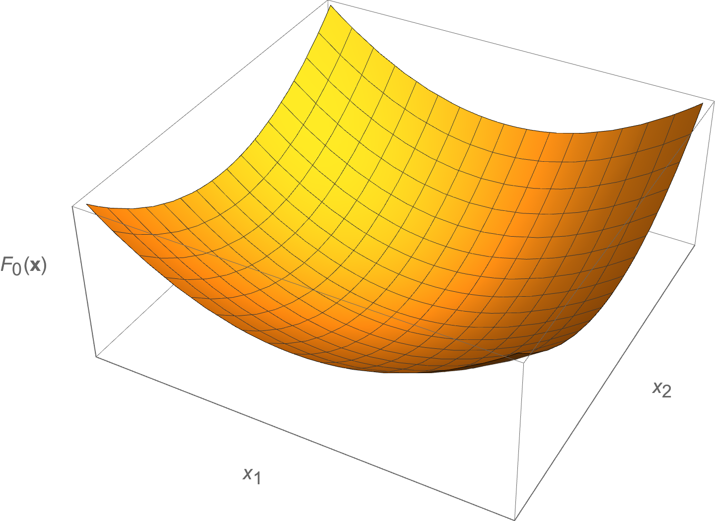
fig. 1. Convex objective function.
- A convex objective looks like a bowl, “holds water”.
- If connect two feasible points line segment in the ? above bottom of the bowl.
A non-convex function is illustrated in fig. 2, which has a number of local minimums.
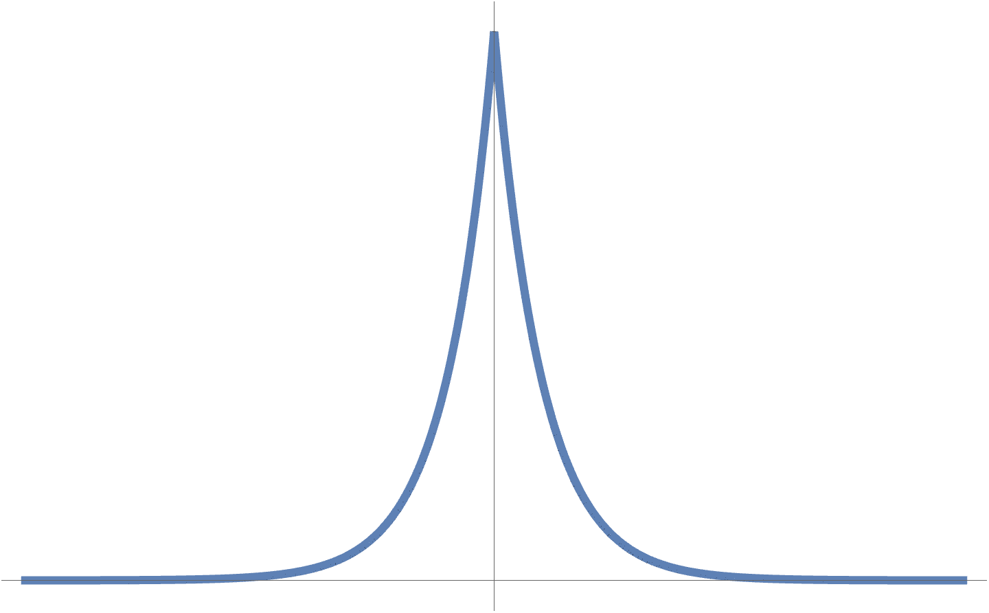
fig. 2. Non-convex (wavy) figure with a number of local minimums.
Example: Line fitting.
A linear fit of some points distributed around a line \( y = a x + b \) is plotted in fig. 3. Here \( a, b \) are the optimization variables \( \Bx = (a, b) \).
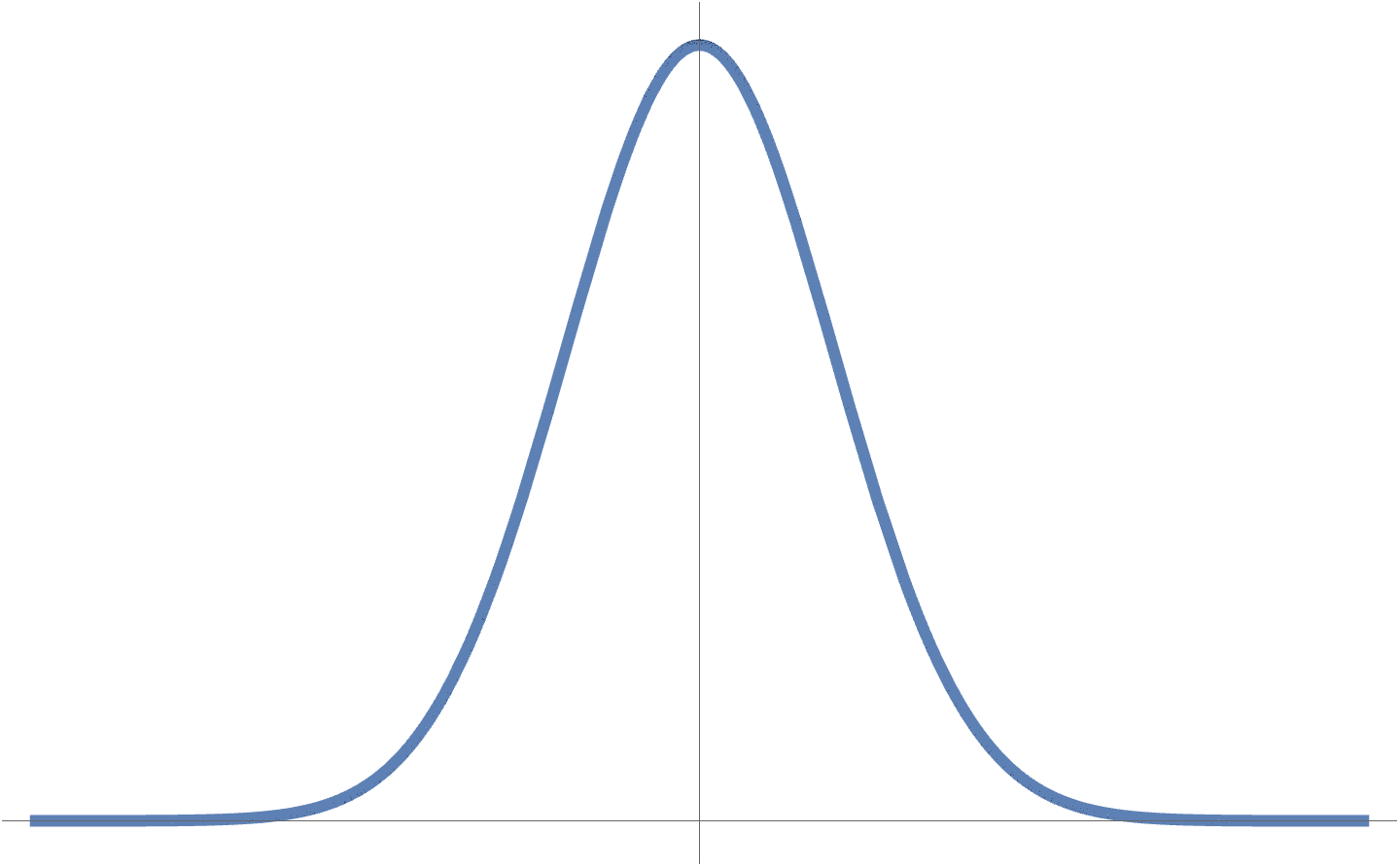
fig. 3. Linear fit of points around a line.
How is the solution for such a best fit line obtained?
Approach 1: Calculus minimization of a multivariable error function.
Describe an error function, describing how far from the line a given point is.
\begin{equation}\label{eqn:intro:100}
y_i – (a x_i + b),
\end{equation}
Because this can be positive or negative, we can define a squared variant of this, and then sum over all data points.
\begin{equation}\label{eqn:intro:120}
F_0 = \sum_{i=1}^n \lr{ y_i – (a x_i + b) }^2.
\end{equation}
One way to solve (for \( a, b \)): Take the derivatives
\begin{equation}\label{eqn:intro:140}
\begin{aligned}
\PD{a}{F_0} &= \sum_{i=1}^n 2 ( y_i – (a x_i + b) )(-x_i) = 0 \\
\PD{b}{F_0} &= \sum_{i=1}^n 2 ( y_i – (a x_i + b) )(-1) = 0.
\end{aligned}
\end{equation}
This yields
\begin{equation}\label{eqn:intro:160}
\begin{aligned}
\sum_{i = 1}^n y_i &= \lr{\sum_{i = 1}^n x_i} a + \lr{\sum_{i = 1}^n 1} b \\
\sum_{i = 1}^n x_i y_i &= \lr{\sum_{i = 1}^n x_i^2} a + \lr{\sum_{i = 1}^n x_i} b.
\end{aligned}
\end{equation}
In matrix form, this is
\begin{equation}\label{eqn:intro:180}
\begin{bmatrix}
\sum x_i y_i \\
\sum y_i
\end{bmatrix}
=
\begin{bmatrix}
\sum x_i^2 & \sum x_i \\
\sum x_i & n
\end{bmatrix}
\begin{bmatrix}
a \\
b
\end{bmatrix}.
\end{equation}
If invertible, have an analytic solution for \( (a^\conj, b^\conj) \). This is a convex optimization problem because \( F(x) = x^2 \) is a convex “quadratic program”. In general a quadratic program has the structure
\begin{equation}\label{eqn:intro:200}
F(a, b) = (\cdots) a^2 + (\cdots) a b + (\cdots) b^2.
\end{equation}
Approach 2: Linear algebraic formulation.
\begin{equation}\label{eqn:intro:220}
\begin{bmatrix}
y_1 \\
\vdots \\
y_n
\end{bmatrix}
=
\begin{bmatrix}
x_1 & 1 \\
\vdots & \vdots \\
x_n & 1
\end{bmatrix}
\begin{bmatrix}
a \\
b
\end{bmatrix}
+
\begin{bmatrix}
z_1 \\
\vdots \\
z_n
\end{bmatrix}
,
\end{equation}
or
\begin{equation}\label{eqn:intro:240}
\By = H \Bv + \Bz,
\end{equation}
where \( \Bz \) is the error vector. The problem is now reduced to to: Fit \( \By \) to be as close to \( H \Bv + \Bz \) as possible, or to minimize the norm of the error vector, or
\begin{equation}\label{eqn:intro:260}
\begin{aligned}
\min_\Bv \Norm{ \By – H \Bv }^2_2
&= \min_\Bv \lr{ \By – H \Bv }^\T \lr{ \By – H \Bv } \\
&= \min_\Bv
\lr{ \By^\T \By – \By^\T H \Bv – \Bv^\T H \By + \Bv^\T H^\T H \Bv } \\
&= \min_\Bv
\lr{ \By^\T \By – 2 \By^\T H \Bv + \Bv^\T H^\T H \Bv }.
\end{aligned}
\end{equation}
It is now possible to take the derivative with respect to the \( \Bv \) vector (i.e. the gradient with respect to the coordinates of the constraint vector)
\begin{equation}\label{eqn:intro:280}
\PD{\Bv}{}
\lr{ \By^\T \By – 2 \By^\T H \Bv + \Bv^\T H^\T H \Bv }
=
– 2 \By^\T H + 2 \Bv^\T H^\T H
= 0,
\end{equation}
or
\begin{equation}\label{eqn:intro:300}
(H^\T H) \Bv = H^\T \By,
\end{equation}
so, assuming that \( H^\T H \) is invertible, the optimization problem has solution
\begin{equation}\label{eqn:intro:320}
\Bv^\conj =
(H^\T H)^{-1} H^\T \By,
\end{equation}
where
\begin{equation}\label{eqn:intro:340}
\begin{aligned}
H^\T H
&=
\begin{bmatrix}
x_1 & \cdots & x_n \\
1 & \cdots & 1 \\
\end{bmatrix}
\begin{bmatrix}
x_1 & 1 \\
\vdots & \vdots \\
x_n & 1
\end{bmatrix} \\
&=
\begin{bmatrix}
\sum x_i^2 & \sum x_i \\
\sum x_i & n
\end{bmatrix}
,
\end{aligned}
\end{equation}
as seen in the calculus approach.
Maximum Likelyhood Estimation (MLE).
It is reasonable to ask why the 2-norm was picked for the objective function?
- One justification is practical: Because we can solve the derivative equation.
- Another justification: In statistics the error vector \( \Bz = \By – H \Bv \) can be modelled as an IID (Independently and Identically Distributed) Gaussian random variable (i.e. noise). Under this model, the use of the 2-norm can be viewed as a consequence of such an ML estimation problem (see [1] ch. 7).
A Gaussian fig. 4 IID model is given by
\begin{equation}\label{eqn:intro:360}
y_i = a x_i + b
\end{equation}
\begin{equation}\label{eqn:intro:380}
z_i = y_i – a x_i -b \sim N(O, O^2)
\end{equation}
\begin{equation}\label{eqn:intro:400}
P_Z(z) = \inv{\sqrt{2 \pi \sigma}} \exp\lr{ -\inv{2} z^2/\sigma^2 }.
\end{equation}
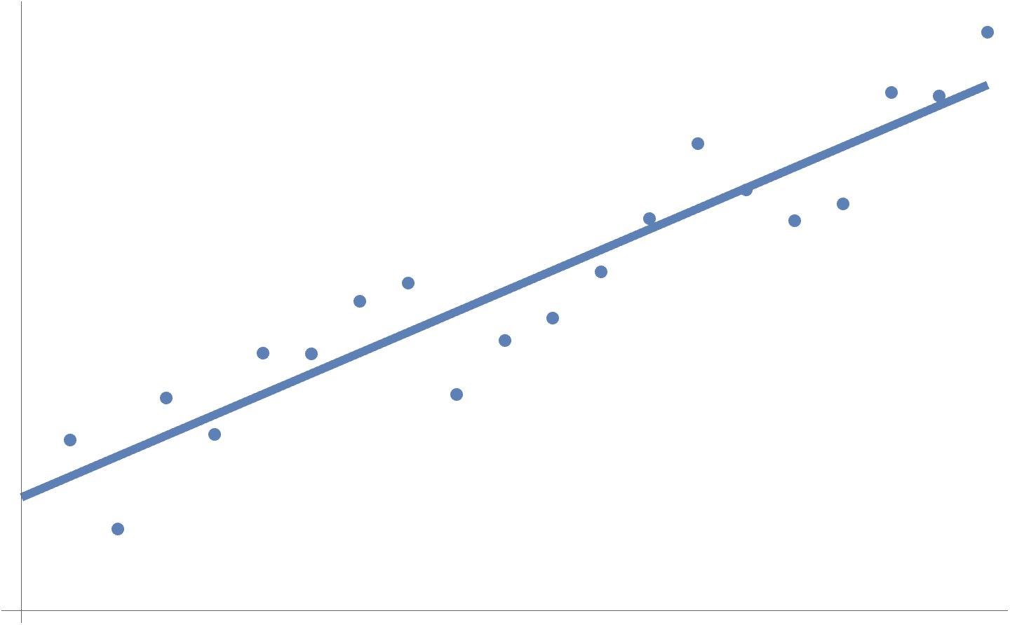
fig. 4. Gaussian probability distribution.
MLE: Maximum Likelyhood Estimator
Pick \( (a,b) \) to maximize the probability of observed data.
\begin{equation}\label{eqn:intro:420}
\begin{aligned}
(a^\conj, b^\conj)
&= \arg \max P( x, y ; a, b ) \\
&= \arg \max P_Z( y – (a x + b) ) \\
&= \arg \max \prod_{i = 1}^n \\
&= \arg \max \inv{\sqrt{2 \pi \sigma}} \exp\lr{ -\inv{2} (y_i – a x_i – b)^2/\sigma^2 }.
\end{aligned}
\end{equation}
Taking logs gives
\begin{equation}\label{eqn:intro:440}
\begin{aligned}
(a^\conj, b^\conj)
&= \arg \max
\lr{
\textrm{constant}
-\inv{2} \sum_i (y_i – a x_i – b)^2/\sigma^2
} \\
&= \arg \min
\inv{2} \sum_i (y_i – a x_i – b)^2/\sigma^2 \\
&= \arg \min
\sum_i (y_i – a x_i – b)^2/\sigma^2
\end{aligned}
\end{equation}
Here \( \arg \max \) is not the maximum of the function, but the value of the parameter (the argument) that maximizes the function.
Double sides exponential noise
A double sided exponential distribution is plotted in fig. 5, and has the mathematical form
\begin{equation}\label{eqn:intro:460}
P_Z(z) = \inv{2 c} \exp\lr{ -\inv{c} \Abs{z} }.
\end{equation}
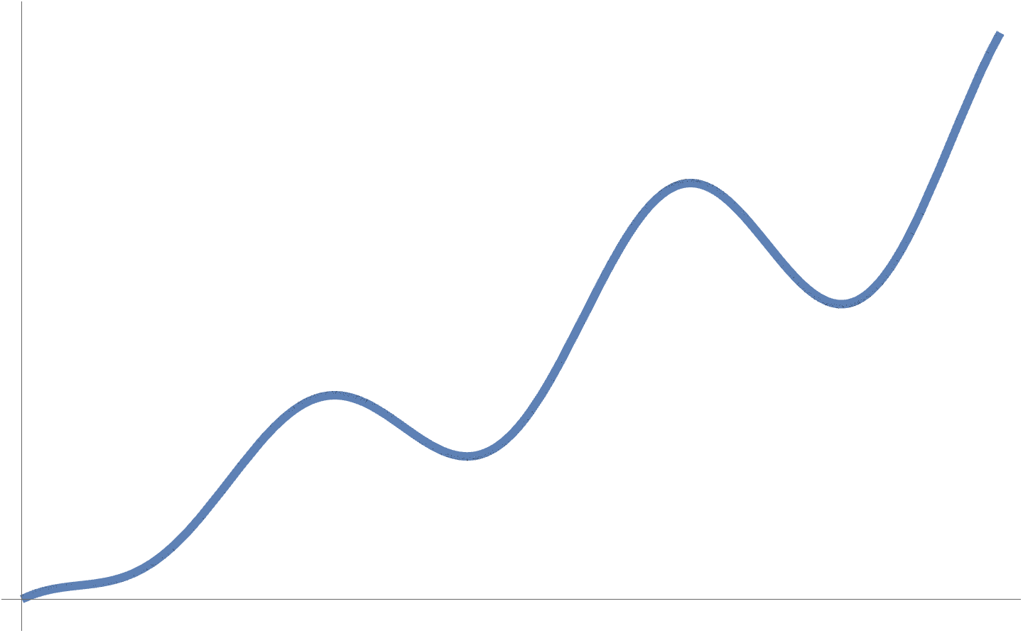
fig. 5. Double sided exponential probability distribution.
The optimization problem is
\begin{equation}\label{eqn:intro:480}
\begin{aligned}
\max_{a,b} \prod_{i = 1}^n P_z(z_i)
&=
\max_{a,b} \prod_{i = 1}^n
\inv{2 c} \exp\lr{ -\inv{c} \Abs{z_i} } \\
&=
\max_{a,b} \prod_{i = 1}^n
\inv{2 c} \exp\lr{ -\inv{c} \Abs{y_i – a x_i – b} } \\
&=
\max_{a,b}
\lr{\inv{2 c}}^n \exp\lr{ -\inv{c} \sum_{i=1}^n \Abs{y_i – a x_i – b} }.
\end{aligned}
\end{equation}
This is a L1 norm problem
\begin{equation}\label{eqn:intro:500}
\min_{a,b} \sum_{i = 1}^n \Abs{ y_i – a x_i – b }.
\end{equation}
i.e.
\begin{equation}\label{eqn:intro:520}
\min_\Bv \Norm{ \By – H \Bv }_1.
\end{equation}
This is still convex, but has no analytic solution, and
is an example of a linear program.
Solution of linear program
Introduce helper variables \( t_1, \cdots, t_n \), and minimize \( \sum_i t_i \), such that
\begin{equation}\label{eqn:intro:540}
\Abs{ y_i – a x_i – b } \le t_i,
\end{equation}
This is now an optimization problem for \( a, b, t_1, \cdots t_n \). A linear program is defined as
\begin{equation}\label{eqn:intro:560}
\min_{a, b, t_1, \cdots t_n} \sum_i t_i
\end{equation}
such that
\begin{equation}\label{eqn:intro:580}
\begin{aligned}
y_i – a x_i – b \le t_i
y_i – a x_i – b \ge -t_i
\end{aligned}
\end{equation}
Single sided exponential
What if your noise doesn’t look double sided, with only noise for values \( x > 0 \). Can define a single sided probability distribution, as that of fig. 6.
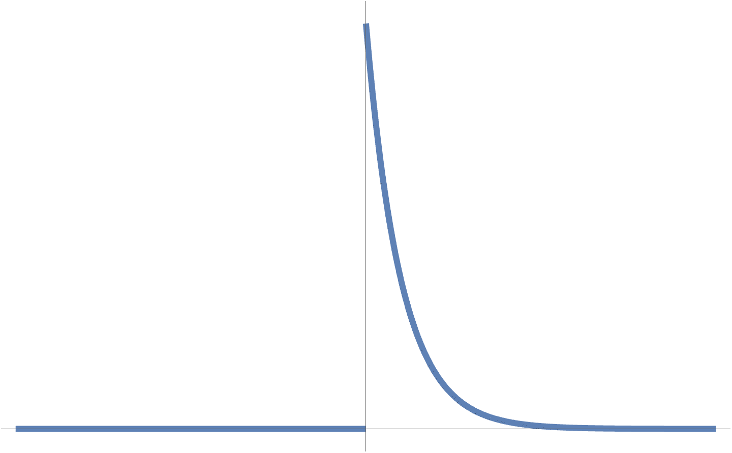
fig. 6. Single sided exponential distribution.
\begin{equation}\label{eqn:intro:600}
P_Z(z) =
\left\{
\begin{array}{l l}
\inv{c} e^{-z/c} & \quad \mbox{\( z \ge 0 \)} \\
0 & \quad \mbox{\( z < 0 \)} \end{array} \right. \end{equation} i.e. all \( z_i \) error values are always non-negative. \begin{equation}\label{eqn:intro:620} \log P_z(z) = \left\{ \begin{array}{l l} \textrm{const} – z/c & \quad \mbox{\( z > 0\)} \\
-\infty & \quad \mbox{\( z< 0\)}
\end{array}
\right.
\end{equation}
Problem becomes
\begin{equation}\label{eqn:intro:640}
\min_{a, b} \sum_i \lr{ y_i – a x_i – b }
\end{equation}
such that
\begin{equation}\label{eqn:intro:660}
y_i – a x_i – b \ge t_i \qquad \forall i
\end{equation}
Uniform noise
For noise that is uniformly distributed in a range, as that of fig. 7, which is constant in the range \( [-c,c] \) and zero outside that range.
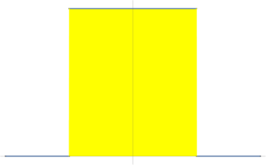
fig. 7. Uniform probability distribution.
\begin{equation}\label{eqn:intro:680}
P_Z(z) =
\left\{
\begin{array}{l l}
\inv{2 c} & \quad \mbox{\( \Abs{z} \le c\)} \\
0 & \quad \mbox{\( \Abs{z} > c. \)}
\end{array}
\right.
\end{equation}
or
\begin{equation}\label{eqn:intro:700}
\log P_Z(z) =
\left\{
\begin{array}{l l}
\textrm{const} & \quad \mbox{\( \Abs{z} \le c\)} \\
-\infty & \quad \mbox{\( \Abs{z} > c. \)}
\end{array}
\right.
\end{equation}
MLE solution
\begin{equation}\label{eqn:intro:720}
\max_{a,b} \prod_{i = 1}^n P(x, y; a, b)
=
\max_{a,b} \sum_{i = 1}^n \log P_Z( y_i – a x_i – b )
\end{equation}
Here the argument is constant if \( -c \le y_i – a x_i – b \le c \), so an ML solution is \underline{any} \( (a,b) \) such that
\begin{equation}\label{eqn:intro:740}
\Abs{ y_i – a x_i – b } \le c \qquad \forall i \in 1, \cdots, n.
\end{equation}
This is a linear program known as a “feasibility problem”.
\begin{equation}\label{eqn:intro:760}
\min d
\end{equation}
such that
\begin{equation}\label{eqn:intro:780}
\begin{aligned}
y_i – a x_i – b &\le d \\
y_i – a x_i – b &\ge -d
\end{aligned}
\end{equation}
If \( d^\conj \le c \), then the problem is feasible, however, if \( d^\conj > c \) it is infeasible.
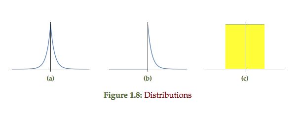
Method comparison
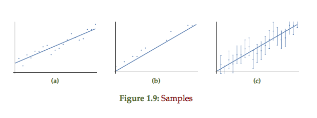
The double sided exponential, single sided exponential and uniform probability distributions of fig 1.8 each respectively represent the point plots of the form fig 1.9. The double sided exponential samples are distributed on both sides of the line, the single sided strictly above or on the line, and the uniform representing error bars distributed around the line of best fit.
References
[1] Stephen Boyd and Lieven Vandenberghe. Convex optimization. Cambridge university press, 2004.