[Click here for a PDF of this post with nicer formatting]

Disclaimer

Peeter’s lecture notes from class. These may be incoherent and rough.

Residual for LMS methods

Mostly on slides:

12_ODS.pdf

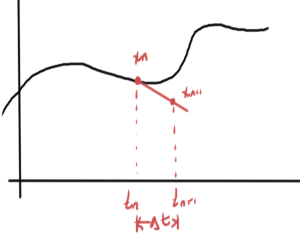
Residual is illustrated in fig. 1, assuming that the iterative method was accurate until \( t_{n} \)

fig. 1. Residual illustrated

Summary

• [FE]: \( R_{n+1} \sim \lr{ \Delta t}^2 \). This is of order \( p = 1 \).
• [BE]: \( R_{n+1} \sim \lr{ \Delta t}^2 \). This is of order \( p = 1 \).
• [TR]: \( R_{n+1} \sim \lr{ \Delta t}^3 \). This is of order \( p = 2 \).
• [BESTE]: \( R_{n+1} \sim \lr{ \Delta t}^4 \). This is of order \( p = 3 \).

Global error estimate

Suppose \( t \in [0, 1] s \), with \( N = 1/{\Delta t} \) intervals. For a method with local error of order \( R_{n+1} \sim \lr{ \Delta t}^2 \) the global error is approximately \( N R_{n+1} \sim \Delta t \).

Stability

Recall that a linear multistep method (LMS) was a system of the form

\begin{equation}\label{eqn:multiphysicsL16:20}
\sum_{j=-1}^{k-1} \alpha_j x_{n-j} = \Delta t \sum_{j=-1}^{k-1} \beta_j f( x_{n-j}, t_{n-j} )
\end{equation}

Consider a one dimensional test problem

\begin{equation}\label{eqn:multiphysicsL16:40}
\dot{x}(t) = \lambda x(t)
\end{equation}

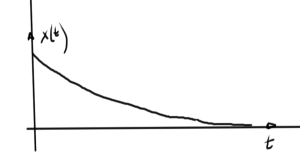
where as in fig. 2, \( \Re(\lambda) < 0 \) is assumed to ensure stability.

fig. 2. Stable system

Linear stability theory can be thought of as asking the question: “Is the solution of \ref{eqn:multiphysicsL16:40} computed by my LMS method also stable?”

Application of \ref{eqn:multiphysicsL16:20} to \ref{eqn:multiphysicsL16:40} gives

\begin{equation}\label{eqn:multiphysicsL16:60}
\sum_{j=-1}^{k-1} \alpha_j x_{n-j} = \Delta t \sum_{j=-1}^{k-1} \beta_j \lambda x_{n-j},
\end{equation}

or
\begin{equation}\label{eqn:multiphysicsL16:80}
\sum_{j=-1}^{k-1} \lr{ \alpha_j – \Delta \beta_j \lambda }
x_{n-j} = 0.
\end{equation}

With

\begin{equation}\label{eqn:multiphysicsL16:100}
\gamma_j = \alpha_j – \Delta \beta_j \lambda,
\end{equation}

this expands to
\begin{equation}\label{eqn:multiphysicsL16:120}
\gamma_{-1} x_{n+1}
+
\gamma_{0} x_{n}
+
\gamma_{1} x_{n-1}
+
\cdots
+
\gamma_{k-1} x_{n-k} .
\end{equation}

This can be seen as a

• discrete time system
• FIR filter

The numerical solution \( x_n \) will be stable if \ref{eqn:multiphysicsL16:120} is stable.

A characteristic equation associated with \ref{eqn:multiphysicsL16:120} can be defined as

\begin{equation}\label{eqn:multiphysicsL16:140}
\gamma_{-1} z^k
+
\gamma_{0} z^{k-1}
+
\gamma_{1} z^{k-2}
+
\cdots
+
\gamma_{k-1} = 0.
\end{equation}

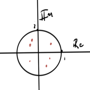
This is a polynomial with roots \( z_n \) (poles). This is stable if the poles satisfy \( \Abs{z_n} < 1 \), as illustrated in fig. 3

Stability

Observe that the \( \gamma’s \) are dependent on \( \Delta t \).

FIXME: There’s a lot of handwaving here that could use more strict justification. Check if the text covers this in more detail.

Example: Forward Euler stability

For \( k = 1 \) step.

\begin{equation}\label{eqn:multiphysicsL16:180}
x_{n+1} – x_n = \Delta t f( x_n, t_n ),
\end{equation}

the coefficients are \( \alpha_{-1} = 1, \alpha_0 = -1, \beta_{-1} = 0, \beta_0 =1 \). For the simple function above

\begin{equation}\label{eqn:multiphysicsL16:200}
\gamma_{-1} = \alpha_{-1} – \Delta t \lambda \beta_{-1} = 1
\end{equation}
\begin{equation}\label{eqn:multiphysicsL16:220}
\gamma_{0} = \alpha_{0} – \Delta t \lambda \beta_{0} = -1 – \Delta t \lambda.
\end{equation}

The stability polynomial is

\begin{equation}\label{eqn:multiphysicsL16:240}
1 z + \lr{ -1 – \Delta t \lambda} = 0,
\end{equation}

or

\begin{equation}\label{eqn:multiphysicsL16:260}
\boxed{
z = 1 + \delta t \lambda.
}
\end{equation}

This is the root, or pole.

For stability we must have

\begin{equation}\label{eqn:multiphysicsL16:280}
\Abs{ 1 + \Delta t \lambda } < 1,
\end{equation}

or
\begin{equation}\label{eqn:multiphysicsL16:300}
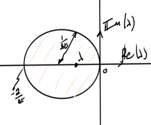
\Abs{ \lambda – \lr{ -\inv{\Delta t} } } < \inv{\Delta t},
\end{equation}

This inequality is illustrated roughly in fig. 4.

fig. 4. Stability region of FE

All poles of my system must be inside the stability region in order to get stable \( \gamma \).