[Click here for a PDF of this post with nicer formatting]
In class today was a highlight of stability methods for linear multistep methods. To motivate the methods used, it is helpful to take a step back and review stability concepts for LDE systems.
By way of example, consider a second order LDE homogeneous system defined by
\begin{equation}\label{eqn:stabilityLDEandDiscreteTime:20}
\frac{d^2 x}{dt^2} + 3 \frac{dx}{dt} + 2 = 0.
\end{equation}
Such a system can be solved by assuming an exponential solution, say
\begin{equation}\label{eqn:stabilityLDEandDiscreteTime:40}
x(t) = e^{s t}.
\end{equation}
Substitution gives
\begin{equation}\label{eqn:stabilityLDEandDiscreteTime:60}
e^{st} \lr{ s^2 + 3 s + 2 } = 0,
\end{equation}
The polynomial part of this equation, the characteristic equation has roots \( s = -2, -1 \).
The general solution of \ref{eqn:stabilityLDEandDiscreteTime:20} is formed by a superposition of solutions for each value of \(s\)
\begin{equation}\label{eqn:stabilityLDEandDiscreteTime:80}
x(t) = a e^{-2 t} + b e^{-t}.
\end{equation}
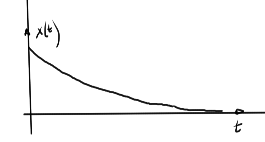
Independent of any selection of the superposition constants \( a, b \), this function will not blow up as \( t \rightarrow \infty \).
This “stability” is due to the fact that both of the characteristic equation roots lie in the left hand Argand plane.
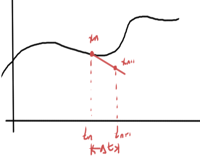
Now consider a discretized form of this LDE. This will have the form
\begin{equation}\label{eqn:stabilityLDEandDiscreteTime:100}
\begin{aligned}
0 &=
\inv{\lr{\Delta t}^2}
\lr{ x_{n+2} – 2 x_{n-1} + x_n } + \frac{3}{\Delta t} \lr{ x_{n+1} – x_n } + 2
x_n \\
&=
x_{n+2} \lr{
\inv{\lr{\Delta t}^2}
}
+
x_{n+1} \lr{
\frac{3}{\Delta t}
-\frac{2}{\lr{\Delta t}^2}
}
+
x_{n} \lr{
\frac{1}{\lr{\Delta t}^2}
-\frac{3}{\Delta t}
+ 2
},
\end{aligned}
\end{equation}
or
\begin{equation}\label{eqn:stabilityLDEandDiscreteTime:220}
0
=
x_{n+2}
+
x_{n+1} \lr{
3 \Delta t – 2
}
+
x_{n} \lr{
1 – 3 \Delta t + 2 \lr{ \Delta t}^2
}.
\end{equation}
Note that after discretization, each subsequent index corresponds to a time shift. Also observe that the coefficients of this discretized equation are dependent on the discretization interval size \( \Delta t \). If the specifics of those coefficients are ignored, a general form with the following structure can be observed
\begin{equation}\label{eqn:stabilityLDEandDiscreteTime:120}
0 =
x_{n+2} \gamma_0
+
x_{n+1} \gamma_1
+
x_{n} \gamma_2.
\end{equation}
It turns out that, much like the LDE solution by characteristic polynomial, it is possible to attack this problem by assuming a solution of the form
\begin{equation}\label{eqn:stabilityLDEandDiscreteTime:140}
x_n = C z^n.
\end{equation}
A time shift index change \( x_n \rightarrow x_{n+1} \) results in a power adjustment in this assumed solution. This substitution applied to \ref{eqn:stabilityLDEandDiscreteTime:120} yields
\begin{equation}\label{eqn:stabilityLDEandDiscreteTime:160}
0 =
C z^n
\lr{
z^{2} \gamma_0
+
z \gamma_1
+
1 \gamma_2
},
\end{equation}
Suppose that this polynomial has roots \( z \in \{z_1, z_2\} \). A superposition, such as
\begin{equation}\label{eqn:stabilityLDEandDiscreteTime:180}
x_n = a z_1^n + b z_2^n,
\end{equation}
will also be a solution since insertion of this into the RHS of \ref{eqn:stabilityLDEandDiscreteTime:120} yields
\begin{equation}\label{eqn:stabilityLDEandDiscreteTime:200}
a z_1^n
\lr{
z_1^{2} \gamma_0
+
z_1 \gamma_1
+
\gamma_2
}
+
b
z_2^n
\lr{
z_2^{2} \gamma_0
+
z_2 \gamma_1
+
\gamma_2
}
=
a z_1^n \times 0
+b z_2^n \times 0.
\end{equation}
The zero equality follows since \( z_1, z_2 \) are both roots of the characteristic equation for this discretized LDE.
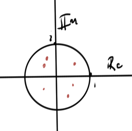
In the discrete \( z \) domain stability requires that the roots satisfy the bound \( \Abs{z} < 1 \), a different stability criteria than in the continuous domain. In fact, there is no a-priori guarantee that stability in the continuous domain will imply stability in the discretized domain.
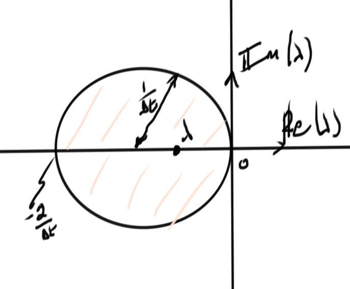
Let's plot those z-domain roots for this example LDE, using \( \Delta t \in \{ 1/2, 1, 2 \} \). The respective characteristic polynomials are
\begin{equation}\label{eqn:stabilityLDEandDiscreteTime:260}
0 = z^2 - \inv{2} z = z \lr{ z - \inv{2} }
\end{equation}
\begin{equation}\label{eqn:stabilityLDEandDiscreteTime:240}
0 = z^2 + z = z\lr{ z + 1 }
\end{equation}
\begin{equation}\label{eqn:stabilityLDEandDiscreteTime:280}
0 = z^2 + 4 z + 3 = (z + 3)(z + 1).
\end{equation}
These have respective roots
\begin{equation}\label{eqn:stabilityLDEandDiscreteTime:300}
z = 0, \inv{2}
\end{equation}
\begin{equation}\label{eqn:stabilityLDEandDiscreteTime:320}
z = 0, -1
\end{equation}
\begin{equation}\label{eqn:stabilityLDEandDiscreteTime:340}
z = -1, -3
\end{equation}
Only the first discretization of these three yields stable solutions in the z domain, although it appears that \( \Delta t = 1 \) is right on the boundary.