References

[Click here for a PDF of this post with nicer formatting]

Disclaimer

Peeter’s lecture notes from class. These may be incoherent and rough.

These are notes for the UofT course PHY1520, Graduate Quantum Mechanics, taught by Prof. Paramekanti.

Where we left off

\begin{equation}\label{eqn:qmLecture9:20}
-i \Hbar \PD{t}{}
\begin{bmatrix}
\psi_1 \\
\psi_2
\end{bmatrix}
=
\begin{bmatrix}
-i \Hbar c \PD{x}{} & m c^2 \\
m c^2 & i \Hbar c \PD{x}{} \\
\end{bmatrix}.
\end{equation}

With a potential this would be

\begin{equation}\label{eqn:qmLecture9:40}
-i \Hbar \PD{t}{}
\begin{bmatrix}
\psi_1 \\
\psi_2
\end{bmatrix}
=
\begin{bmatrix}
-i \Hbar c \PD{x}{} + V(x) & m c^2 \\
m c^2 & i \Hbar c \PD{x}{} + V(x) \\
\end{bmatrix}.
\end{equation}

This means that the potential is raising the energy eigenvalue of the system.

Free Particle

Assuming a form

\begin{equation}\label{eqn:qmLecture9:60}
\begin{bmatrix}
\psi_1(x,t) \\
\psi_2(x,t)
\end{bmatrix}
=
e^{i k x}
\begin{bmatrix}
f_1(t) \\
f_2(t) \\
\end{bmatrix},
\end{equation}

and plugging back into the Dirac equation we have

\begin{equation}\label{eqn:qmLecture9:80}
-i \Hbar \PD{t}{}
\begin{bmatrix}
f_1 \\
f_2
\end{bmatrix}
=
\begin{bmatrix}
k \Hbar c & m c^2 \\
m c^2 & – \Hbar k c \\
\end{bmatrix}
\begin{bmatrix}
f_1 \\
f_2
\end{bmatrix}.
\end{equation}

We can use a diagonalizing rotation

\begin{equation}\label{eqn:qmLecture9:100}
\begin{bmatrix}
f_1 \\
f_2
\end{bmatrix}
=
\begin{bmatrix}
\cos\theta_k & -\sin\theta_k \\
\sin\theta_k & \cos\theta_k \\
\end{bmatrix}
\begin{bmatrix}
f_{+} \\
f_{-} \\
\end{bmatrix}.
\end{equation}

Plugging this in reduces the system to the form

\begin{equation}\label{eqn:qmLecture9:140}
-i \Hbar \PD{t}{}
\begin{bmatrix}
f_{+} \\
f_{-} \\
\end{bmatrix}
=
\begin{bmatrix}
E_k & 0 \\
0 & -E_k
\end{bmatrix}
\begin{bmatrix}
f_{+} \\
f_{-} \\
\end{bmatrix}.
\end{equation}

Where the rotation angle is found to be given by

\begin{equation}\label{eqn:qmLecture9:160}
\begin{aligned}
\sin(2 \theta_k) &= \frac{m c^2}{\sqrt{(\Hbar k c)^2 + m^2 c^4}} \\
\cos(2 \theta_k) &= \frac{\Hbar k c}{\sqrt{(\Hbar k c)^2 + m^2 c^4}} \\
E_k &= \sqrt{(\Hbar k c)^2 + m^2 c^4}
\end{aligned}
\end{equation}

See fig. 1 for a sketch of energy vs momentum. The asymptotes are the limiting cases when \( m c^2 \rightarrow 0 \). The \( + \) branch is what we usually associate with particles. What about the other energy states. For Fermions Dirac argued that the lower energy states could be thought of as “filled up”, using the Pauli principle to leave only the positive energy states available. This was called the “Dirac Sea”. This isn’t a good solution, and won’t work for example for Bosons.

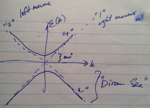
fig. 1. Dirac equation solution space

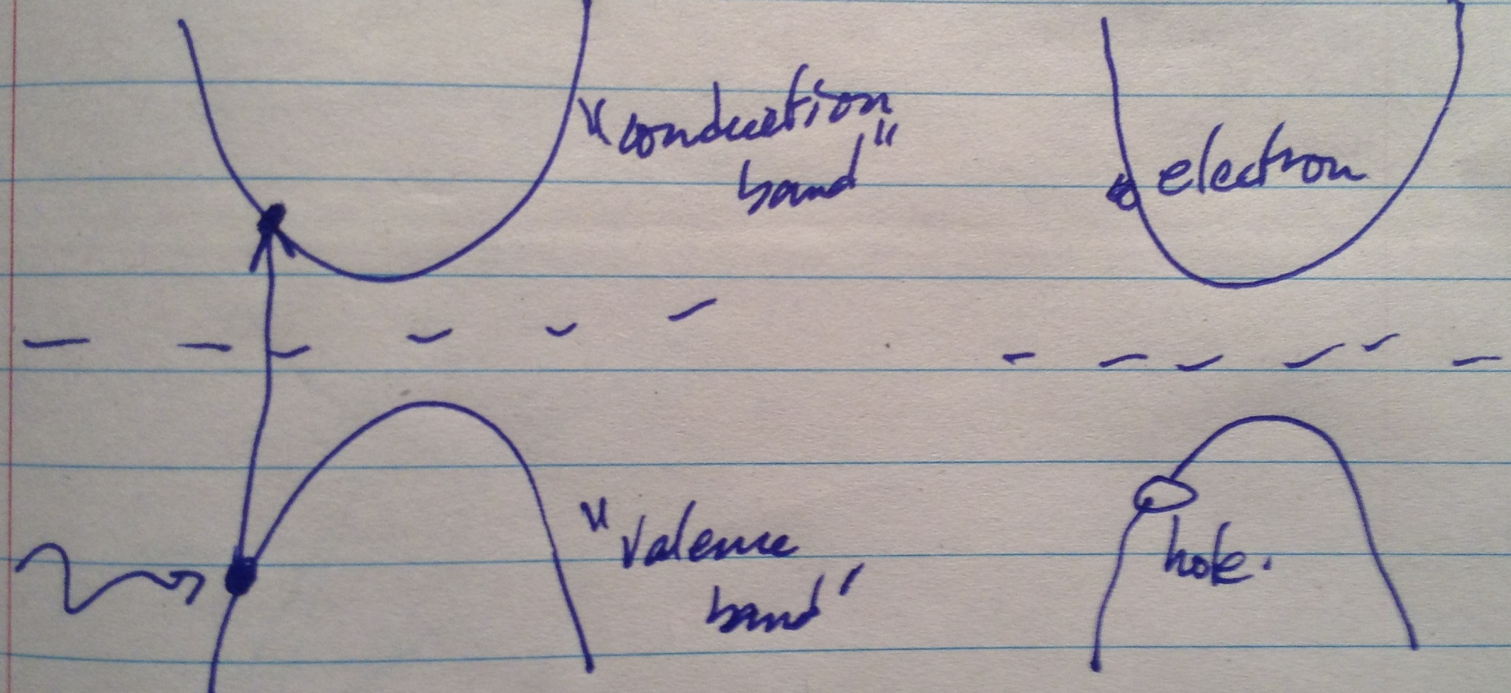
Another way to rationalize this is to employ ideas from solid state theory. For example consider a semiconductor with a valence and conduction band as sketched in fig. 2.

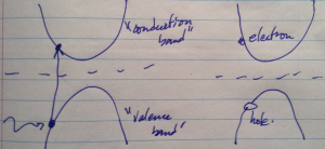
fig. 2. Solid state valence and conduction band transition

A photon can excite an electron from the valence band to the conduction band, leaving all the valence band states filled except for one (a hole). For an electron we can use almost the same picture, as sketched in fig. 3.

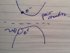
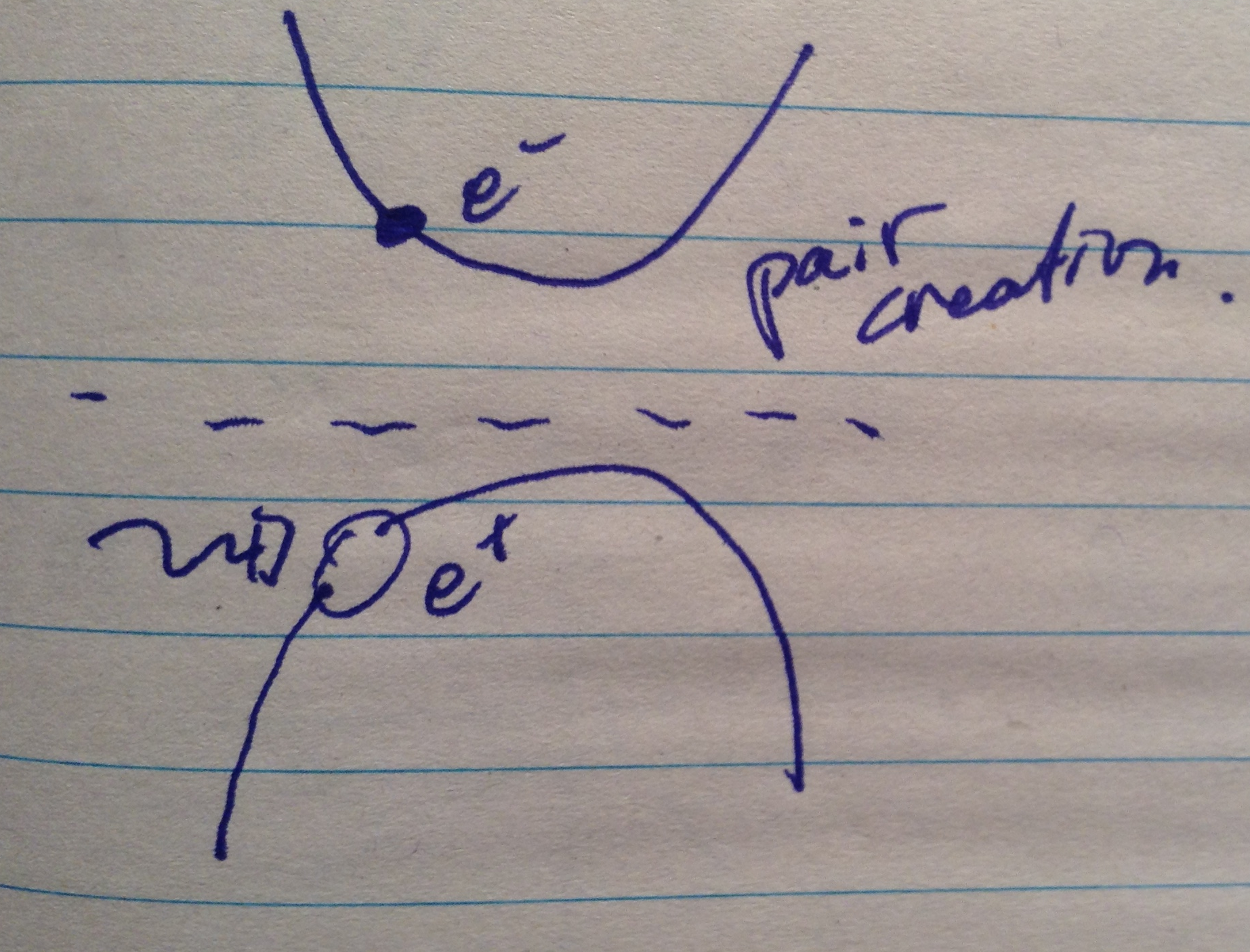
fig. 3. Pair creation

A photon with energy \( E_k – (-E_k) \) can create a positron-electron pair from the vacuum, where the energy of the electron and positron pair is \( E_k \).

At high enough energies, we can see this pair creation occur.

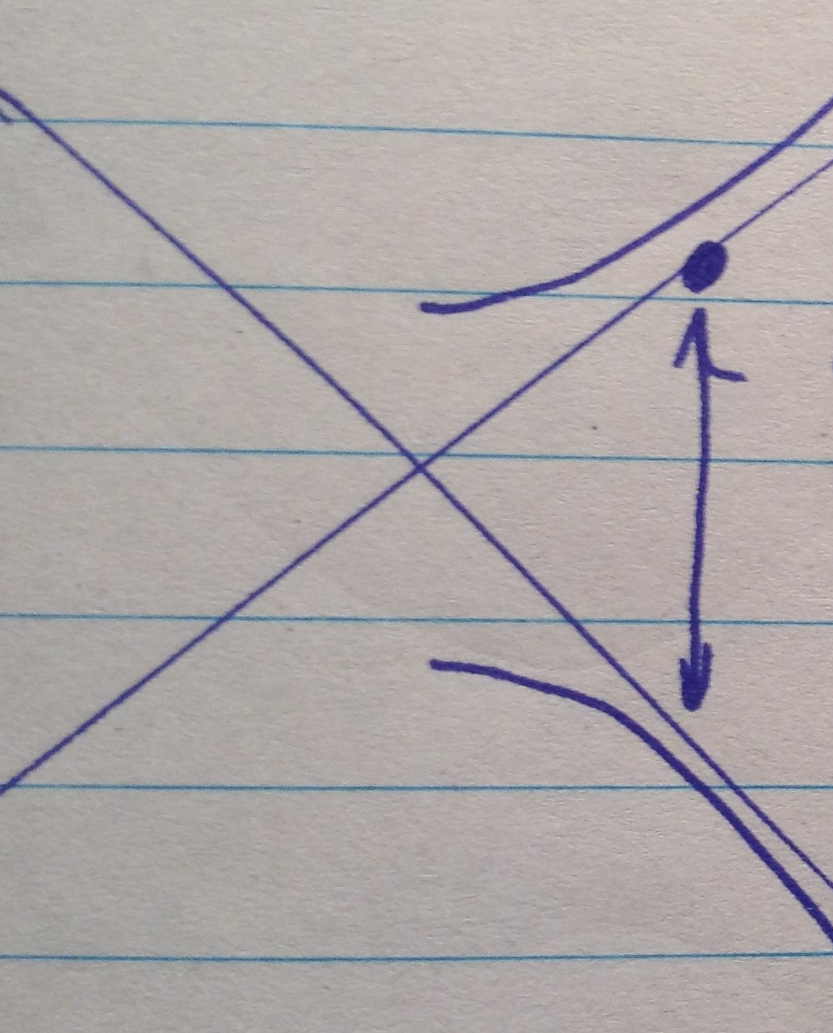
Zitterbewegung

If a particle is created at a non-eigenstate such as one on the asymptotes, then oscillations between the positive and negative branches are possible as sketched in fig. 4.

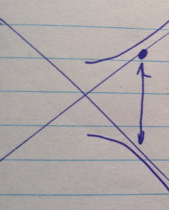
fig. 4. Zitterbewegung oscillation

Only “vertical” oscillations between the positive and negative locations on these branches is possible since those are the points that match the particle momentum. Examining this will be the aim of one of the problem set problems.

Probability and current density

If we define a probability density

\begin{equation}\label{eqn:qmLecture9:180}
\rho(x, t) = \Abs{\psi_1}^2 + \Abs{\psi_2}^2,
\end{equation}

does this satisfy a probability conservation relation

\begin{equation}\label{eqn:qmLecture9:200}
\PD{t}{\rho} + \PD{x}{j} = 0,
\end{equation}

where \( j \) is the probability current. Plugging in the density, we have

\begin{equation}\label{eqn:qmLecture9:220}
\PD{t}{\rho}
=
\PD{t}{\psi_1^\conj} \psi_1
+
\psi_1^\conj \PD{t}{\psi_1}
+
\PD{t}{\psi_2^\conj} \psi_2
+
\psi_2^\conj \PD{t}{\psi_2}.
\end{equation}

It turns out that the probability current has the form

\begin{equation}\label{eqn:qmLecture9:240}
j(x,t) = c \lr{ \psi_1^\conj \psi_1 + \psi_2^\conj \psi_2 }.
\end{equation}

Here the speed of light \( c \) is the slope of the line in the plots above. We can think of this current density as right movers minus the left movers. Any state that is given can be thought of as a combination of right moving and left moving states, neither of which are eigenstates of the free particle Hamiltonian.

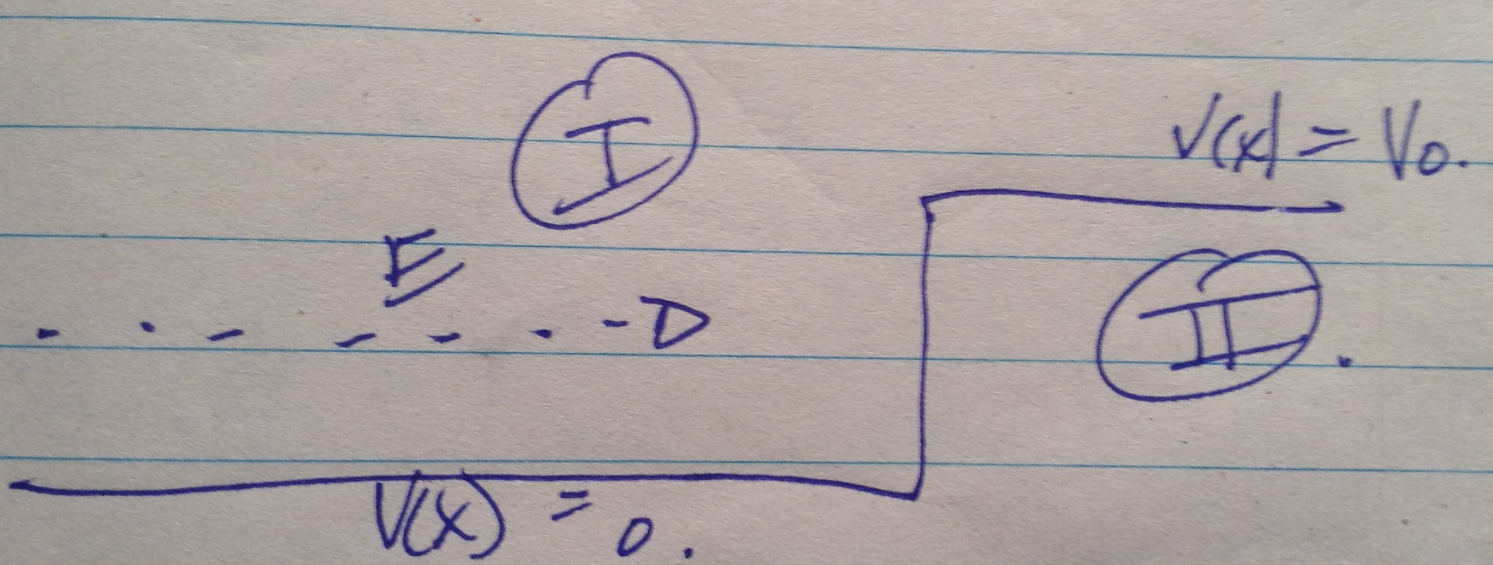
Potential step

The next logical thing to think about, as in non-relativistic quantum mechanics, is to think about what occurs when the particle hits a potential step, as in fig. 5.

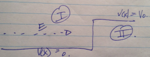
fig. 5. Reflection off a potential barrier

The approach is the same. We write down the wave functions for the \( V = 0 \) region (I), and the higher potential region (II).

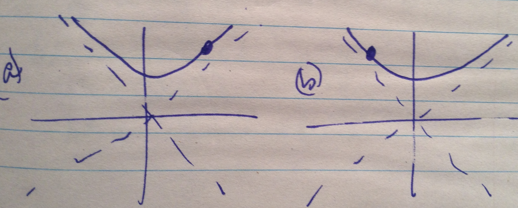
The eigenstates are found on the solid lines above the asymptotes on the right hand movers side as sketched in fig. 6. The right and left moving designations are based on the phase velocity \( \PDi{k}{E} \) (approaching \( \pm c \) on the top-right and top-left quadrants respectively).

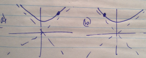
fig. 6. Right movers and left movers

For \( k > 0 \), an eigenstate for the incident wave is

\begin{equation}\label{eqn:qmLecture9:261}
\Bpsi_{\textrm{inc}}(x) =
\begin{bmatrix}
\cos\theta_k \\
\sin\theta_k
\end{bmatrix}
e^{i k x},
\end{equation}

For the reflected wave function, we pick a function on the left moving side of the positive energy branch.

\begin{equation}\label{eqn:qmLecture9:260}
\Bpsi_{\textrm{ref}}(x) =
\begin{bmatrix}
? \\
?
\end{bmatrix}
e^{-i k x},
\end{equation}

We’ll go through this in more detail next time.

Question: Calculate the right going diagonalization

Prove (7).

Answer

To determine the relations for \( \theta_k \) we have to solve

\begin{equation}\label{eqn:qmLecture9:280}
\begin{bmatrix}
E_k & 0 \\
0 & -E_k
\end{bmatrix}
= R^{-1} H R.
\end{equation}

Working with \( \Hbar = c = 1 \) temporarily, and \( C = \cos\theta_k, S = \sin\theta_k \), that is

\begin{equation}\label{eqn:qmLecture9:300}
\begin{aligned}
\begin{bmatrix}
E_k & 0 \\
0 & -E_k
\end{bmatrix}
&=
\begin{bmatrix}
C & S \\
-S & C
\end{bmatrix}
\begin{bmatrix}
k & m \\
m & -k
\end{bmatrix}
\begin{bmatrix}
C & -S \\
S & C
\end{bmatrix} \\
&=
\begin{bmatrix}
C & S \\
-S & C
\end{bmatrix}
\begin{bmatrix}
k C + m S & -k S + m C \\
m C – k S & -m S – k C
\end{bmatrix} \\
&=
\begin{bmatrix}
k C^2 + m S C + m C S – k S^2 & -k S C + m C^2 -m S^2 – k C S \\
-k C S – m S^2 + m C^2 – k S C & k S^2 – m C S -m S C – k C^2
\end{bmatrix} \\
&=
\begin{bmatrix}
k \cos(2 \theta_k) + m \sin(2 \theta_k) & m \cos(2 \theta_k) – k \sin(2 \theta_k) \\
m \cos(2 \theta_k) – k \sin(2 \theta_k) & -k \cos(2 \theta_k) – m \sin(2 \theta_k) \\
\end{bmatrix}.
\end{aligned}
\end{equation}

This gives

\begin{equation}\label{eqn:qmLecture9:320}
\begin{aligned}
E_k
\begin{bmatrix}
1 \\
0
\end{bmatrix}
&=
\begin{bmatrix}
k \cos(2 \theta_k) + m \sin(2 \theta_k) \\
m \cos(2 \theta_k) – k \sin(2 \theta_k) \\
\end{bmatrix} \\
&=
\begin{bmatrix}
k & m \\
m & -k
\end{bmatrix}
\begin{bmatrix}
\cos(2 \theta_k) \\
\sin(2 \theta_k) \\
\end{bmatrix}.
\end{aligned}
\end{equation}

Adding back in the \(\Hbar\)’s and \(c\)’s this is

\begin{equation}\label{eqn:qmLecture9:340}
\begin{aligned}
\begin{bmatrix}
\cos(2 \theta_k) \\
\sin(2 \theta_k) \\
\end{bmatrix}
&=
\frac{E_k}{-(\Hbar k c)^2 -(m c^2)^2}
\begin{bmatrix}
– \Hbar k c & – m c^2 \\
– m c^2 & \Hbar k c
\end{bmatrix}
\begin{bmatrix}
1 \\
0
\end{bmatrix} \\
&=
\inv{E_k}
\begin{bmatrix}
\Hbar k c \\
m c^2
\end{bmatrix}.
\end{aligned}
\end{equation}

Question: Verify the Dirac current relationship.

Prove \ref{eqn:qmLecture9:240}.

Answer

The components of the Schrodinger equation are

\begin{equation}\label{eqn:qmLecture9:360}
\begin{aligned}
-i \Hbar \PD{t}{\psi_1} &= -i \Hbar c \PD{x}{\psi_1} + m c^2 \psi_2 \\
-i \Hbar \PD{t}{\psi_2} &= m c^2 \psi_1 + i \Hbar c \PD{x}{\psi_2},
\end{aligned}
\end{equation}

The conjugates of these are
\begin{equation}\label{eqn:qmLecture9:380}
\begin{aligned}
i \Hbar \PD{t}{\psi_1^\conj} &= i \Hbar c \PD{x}{\psi_1^\conj} + m c^2 \psi_2^\conj \\
i \Hbar \PD{t}{\psi_2^\conj} &= m c^2 \psi_1^\conj – i \Hbar c \PD{x}{\psi_2^\conj}.
\end{aligned}
\end{equation}

This gives
\begin{equation}\label{eqn:qmLecture9:400}
\begin{aligned}
i \Hbar \PD{t}{\rho}
&=
\lr{ i \Hbar c \PD{x}{\psi_1^\conj} + m c^2 \psi_2^\conj } \psi_1 \\
&+ \psi_1^\conj \lr{ i \Hbar c \PD{x}{\psi_1} – m c^2 \psi_2 } \\
&+ \lr{ m c^2 \psi_1^\conj – i \Hbar c \PD{x}{\psi_2^\conj} } \psi_2 \\
&+ \psi_2^\conj \lr{ -m c^2 \psi_1 – i \Hbar c \PD{x}{\psi_2} }.
\end{aligned}
\end{equation}

All the non-derivative terms cancel leaving

\begin{equation}\label{eqn:qmLecture9:420}
\inv{c} \PD{t}{\rho}
=
\PD{x}{\psi_1^\conj} \psi_1
+ \psi_1^\conj \PD{x}{\psi_1}
– \PD{x}{\psi_2^\conj} \psi_2
– \psi_2^\conj \PD{x}{\psi_2}
=
\PD{x}{}
\lr{
\psi_1^\conj \psi_1 –
\psi_2^\conj \psi_2
}.
\end{equation}