[Click here for a PDF of this post with nicer formatting]
Disclaimer
Peeter’s lecture notes from class. These may be incoherent and rough.
These are notes for the UofT course PHY1520, Graduate Quantum Mechanics, taught by Prof. Paramekanti.
Dirac scattering off a potential step
For the non-relativistic case we have
\begin{equation}\label{eqn:qmLecture10:20}
\begin{aligned}
E < V_0 &\Rightarrow T = 0, R = 1 \\ E > V_0 &\Rightarrow T > 0, R < 1.
\end{aligned}
\end{equation}
What happens for a relativistic 1D particle?
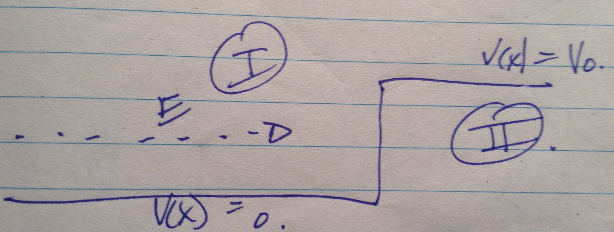
Referring to fig. 1.
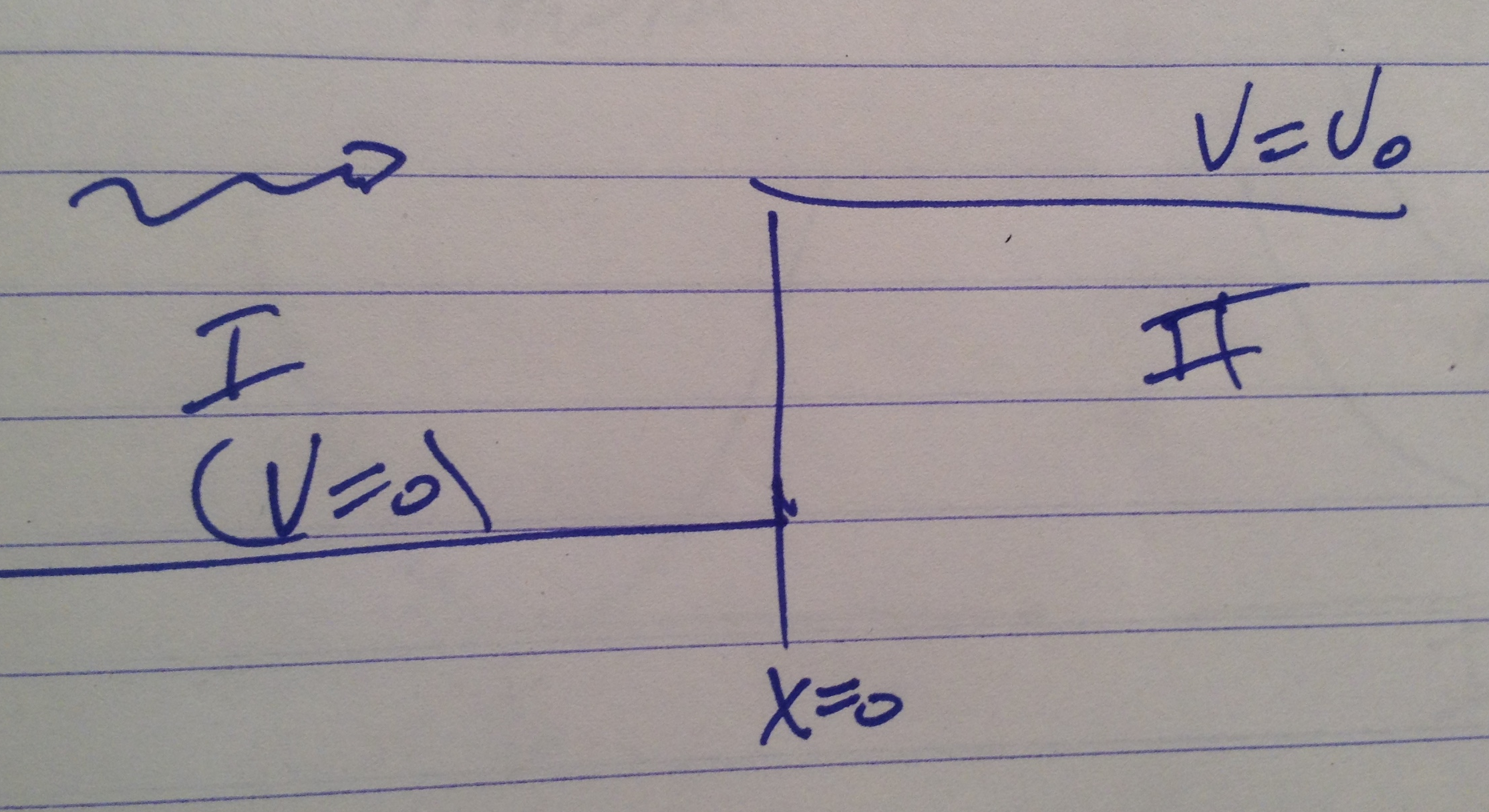
fig. 1. Potential step
the region I Hamiltonian is
\begin{equation}\label{eqn:qmLecture10:40}
H =
\begin{bmatrix}
\hat{p} c & m c^2 \\
m c^2 & – \hat{p} c
\end{bmatrix},
\end{equation}
for which the solution is
\begin{equation}\label{eqn:qmLecture10:60}
\Phi = e^{i k_1 x }
\begin{bmatrix}
\cos \theta_1 \\
\sin \theta_1
\end{bmatrix},
\end{equation}
where
\begin{equation}\label{eqn:qmLecture10:80}
\begin{aligned}
\cos 2 \theta_1 &= \frac{ \Hbar c k_1 }{E_{k_1}} \\
\sin 2 \theta_1 &= \frac{ m c^2 }{E_{k_1}} \\
\end{aligned}
\end{equation}
To consider the \( k_1 < 0 \) case, note that
\begin{equation}\label{eqn:qmLecture10:100}
\begin{aligned}
\cos^2 \theta_1 – \sin^2 \theta_1 &= \cos 2 \theta_1 \\
2 \sin\theta_1 \cos\theta_1 &= \sin 2 \theta_1
\end{aligned}
\end{equation}
so after flipping the signs on all the \( k_1 \) terms we find for the reflected wave
\begin{equation}\label{eqn:qmLecture10:120}
\Phi = e^{-i k_1 x}
\begin{bmatrix}
\sin\theta_1 \\
\cos\theta_1
\end{bmatrix}.
\end{equation}
FIXME: this reasoning doesn’t entirely make sense to me. Make sense of this by trying this solution as was done for the form of the incident wave solution.
The region I wave has the form
\begin{equation}\label{eqn:qmLecture10:140}
\Phi_I
=
A e^{i k_1 x}
\begin{bmatrix}
\cos\theta_1 \\
\sin\theta_1 \\
\end{bmatrix}
+
B e^{-i k_1 x}
\begin{bmatrix}
\sin\theta_1 \\
\cos\theta_1 \\
\end{bmatrix}.
\end{equation}
By the time we are done we want to have computed the reflection coefficient
\begin{equation}\label{eqn:qmLecture10:160}
R =
\frac{\Abs{B}^2}{\Abs{A}^2}.
\end{equation}
The region I energy is
\begin{equation}\label{eqn:qmLecture10:180}
E = \sqrt{ \lr{ m c^2}^2 + \lr{ \Hbar c k_1 }^2 }.
\end{equation}
We must have
\begin{equation}\label{eqn:qmLecture10:200}
E
=
\sqrt{ \lr{ m c^2}^2 + \lr{ \Hbar c k_2 }^2 } + V_0
=
\sqrt{ \lr{ m c^2}^2 + \lr{ \Hbar c k_1 }^2 },
\end{equation}
so
\begin{equation}\label{eqn:qmLecture10:220}
\begin{aligned}
\lr{ \Hbar c k_2 }^2
&=
\lr{ E – V_0 }^2 – \lr{ m c^2}^2 \\
&=
\underbrace{\lr{ E – V_0 + m c }}_{r_1}\underbrace{\lr{ E – V_0 – m c }}_{r_2}.
\end{aligned}
\end{equation}
The \( r_1 \) and \( r_2 \) branches are sketched in fig. 2.
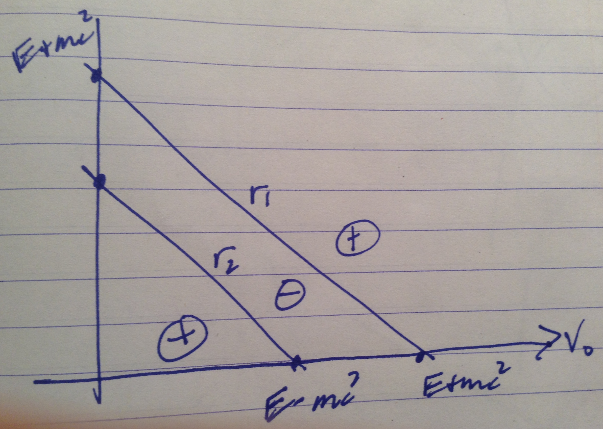
fig. 2. Energy signs
For low energies, we have a set of potentials for which we will have propagation, despite having a potential barrier. For still higher values of the potential barrier the product \( r_1 r_2 \) will be negative, so the solutions will be decaying. Finally, for even higher energies, there will again be propagation.
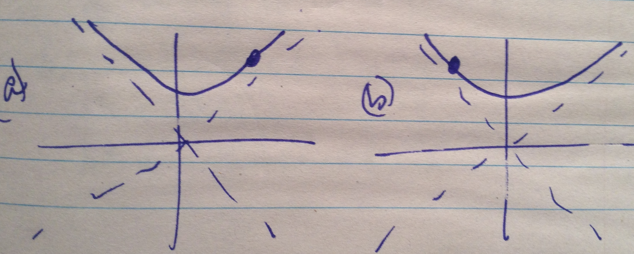
The non-relativistic case is sketched in fig. 3.
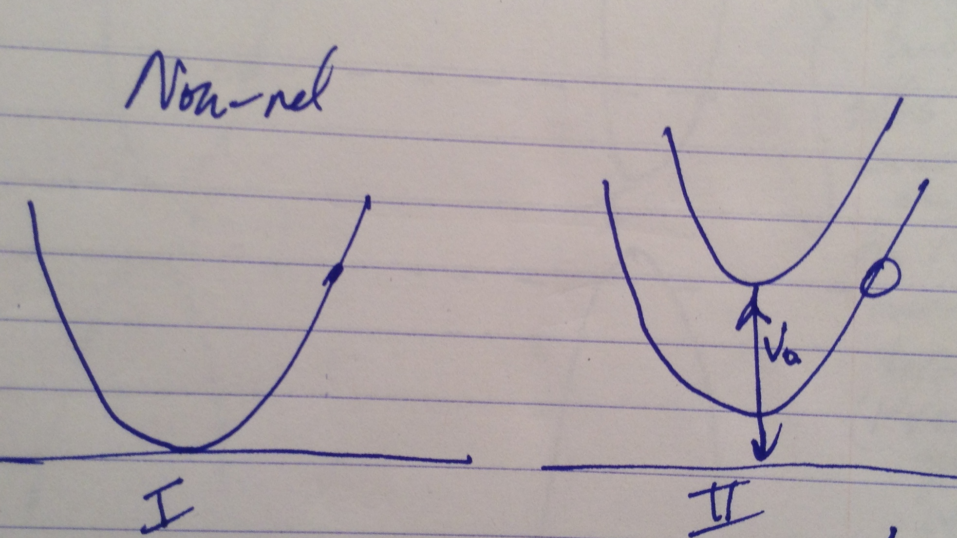
fig. 3. Effects of increasing potential for non-relativistic case
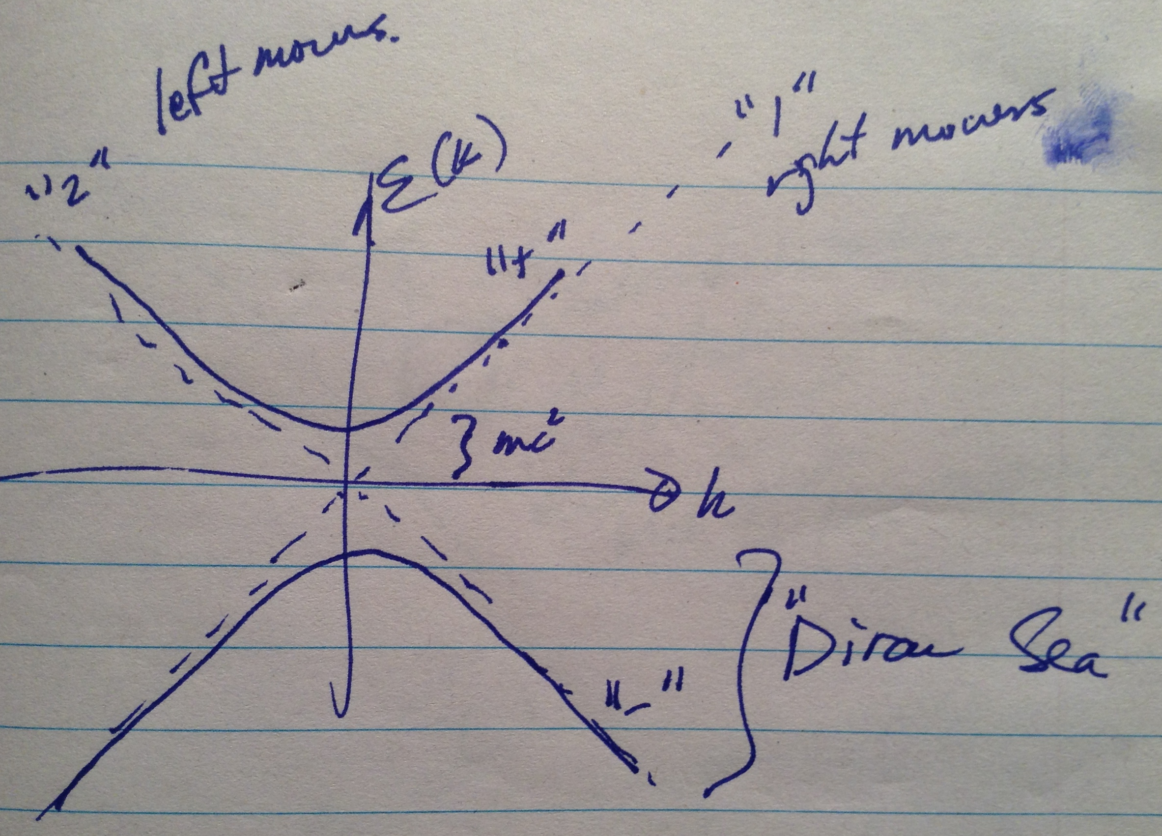
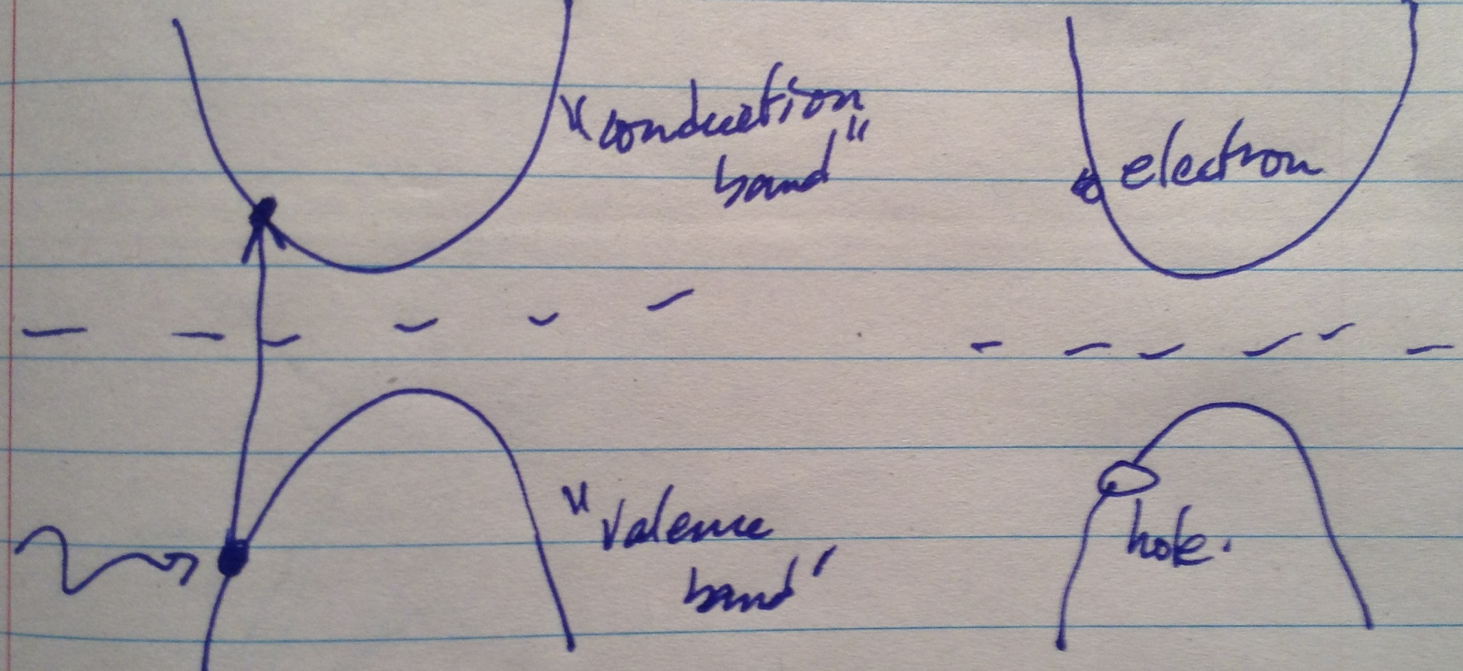
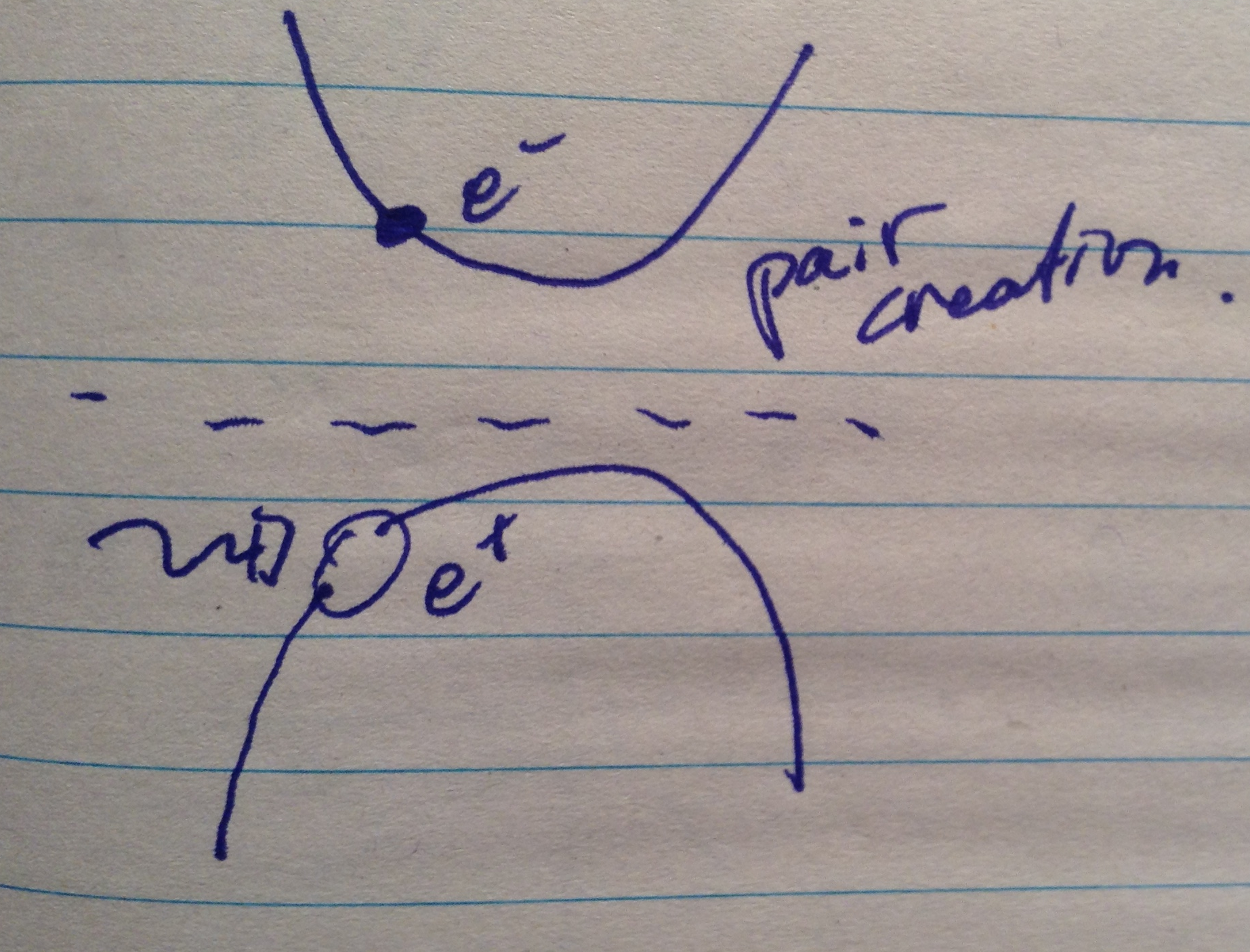
For the relativistic case we must consider three different cases, sketched in fig 4, fig 5, and fig 6 respectively. For the low potential energy, a particle with positive group velocity (what we’ve called right moving) can be matched to an equal energy portion of the potential shifted parabola in region II. This is a case where we have transmission, but no antiparticle creation. There will be an energy region where the region II wave function has only a dissipative term, since there is no region of either of the region II parabolic branches available at the incident energy. When the potential is shifted still higher so that \( V_0 > E + m c^2 \), a positive group velocity in region I with a given energy can be matched to an antiparticle branch in the region II parabolic energy curve.
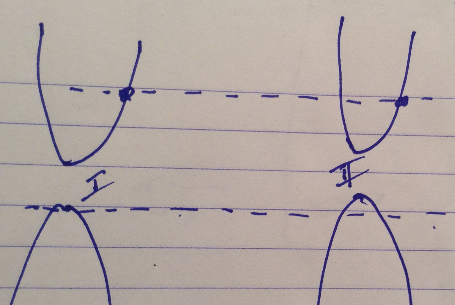
Fig 4. Low potential energy
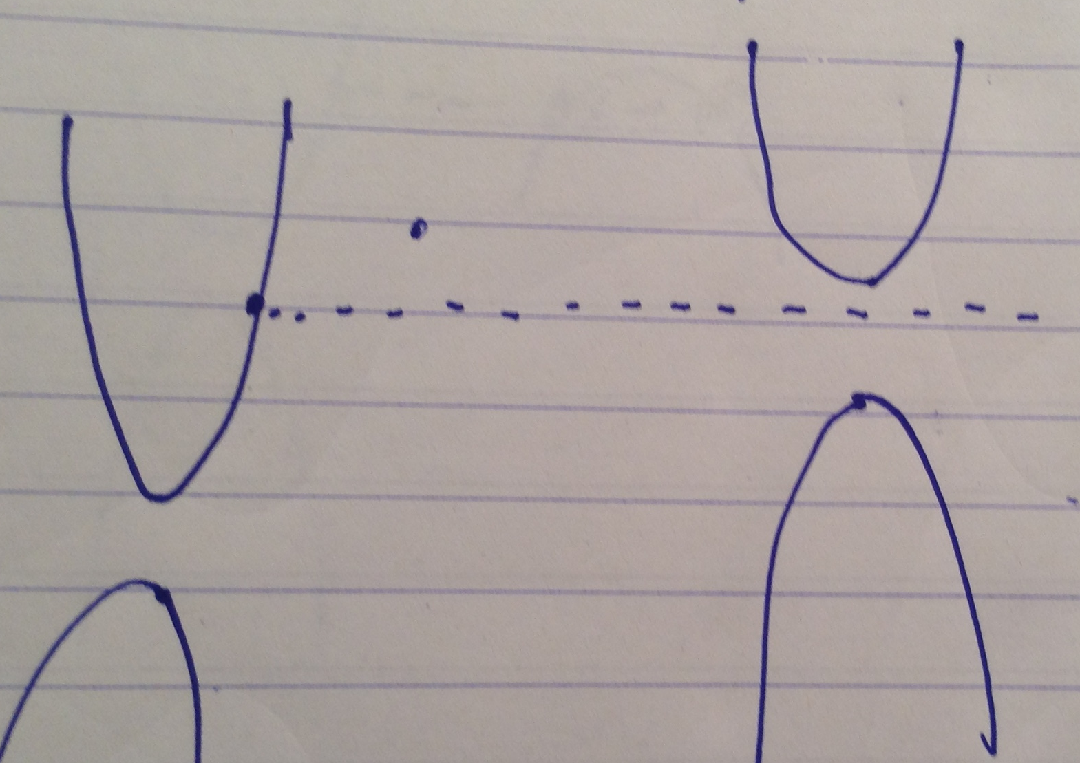
fig. 5. High enough potential energy for no propagation
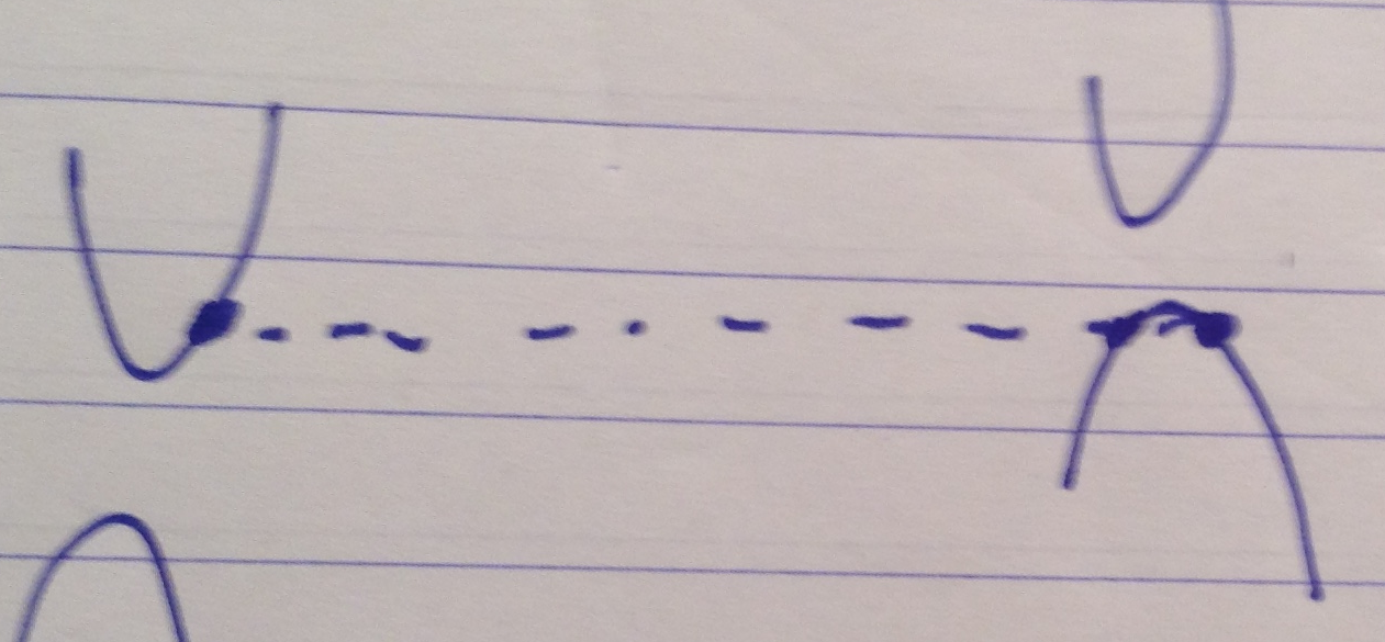
fig 6. High potential energy
Boundary value conditions
We want to ensure that the current across the barrier is conserved (no particles are lost), as sketched in fig. 7.
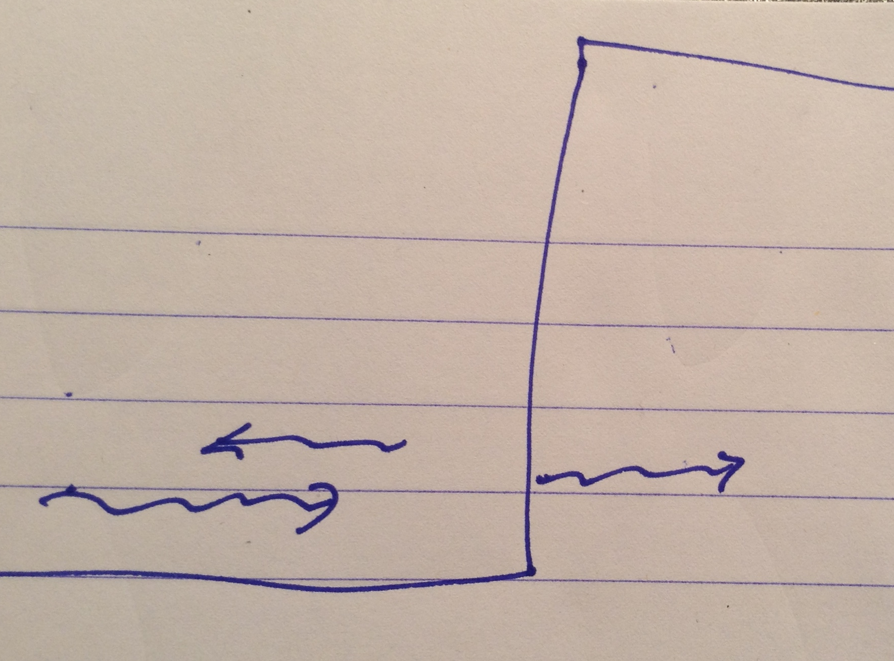
fig. 7. Transmitted, reflected and incident components.
Recall that given a wave function
\begin{equation}\label{eqn:qmLecture10:240}
\Psi =
\begin{bmatrix}
\psi_1 \\
\psi_2
\end{bmatrix},
\end{equation}
the density and currents are respectively
\begin{equation}\label{eqn:qmLecture10:260}
\begin{aligned}
\rho &= \psi_1^\conj \psi_1 + \psi_2^\conj \psi_2 \\
j &= \psi_1^\conj \psi_1 – \psi_2^\conj \psi_2
\end{aligned}
\end{equation}
Matching boundary value conditions requires
- For both the relativistic and non-relativistic cases we must have\begin{equation}\label{eqn:qmLecture10:280}
\Psi_{\textrm{L}} = \Psi_{\textrm{R}}, \qquad \mbox{at \( x = 0 \).}
\end{equation} - For the non-relativistic case we want
\begin{equation}\label{eqn:qmLecture10:300}
\int_{-\epsilon}^\epsilon -\frac{\Hbar^2}{2m} \PDSq{x}{\Psi} =
{\int_{-\epsilon}^\epsilon \lr{ E – V(x) } \Psi(x)}.
\end{equation}The RHS integral is zero, so\begin{equation}\label{eqn:qmLecture10:320}
-\frac{\Hbar^2}{2m} \lr{ \evalbar{\PD{x}{\Psi}}{{\textrm{R}}} – \evalbar{\PD{x}{\Psi}}{{\textrm{L}}} } = 0.
\end{equation}We have to match
For the relativistic case
\begin{equation}\label{eqn:qmLecture10:460}
-i \Hbar \sigma_z \int_{-\epsilon}^\epsilon \PD{x}{\Psi} +
{m c^2 \sigma_x \int_{-\epsilon}^\epsilon \psi}
=
{\int_{-\epsilon}^\epsilon \lr{ E – V_0 } \psi},
\end{equation}
the second two integrals are wiped out, so
\begin{equation}\label{eqn:qmLecture10:340}
-i \Hbar c \sigma_z \lr{ \psi(\epsilon) – \psi(-\epsilon) }
=
-i \Hbar c \sigma_z \lr{ \psi_{\textrm{R}} – \psi_{\textrm{L}} }.
\end{equation}
so we must match
\begin{equation}\label{eqn:qmLecture10:360}
\sigma_z \psi_{\textrm{R}} = \sigma_z \psi_{\textrm{L}} .
\end{equation}
It appears that things are simpler, because we only have to match the wave function values at the boundary, and don’t have to match the derivatives too. However, we have a two component wave function, so there are still two tasks.
Solving the system
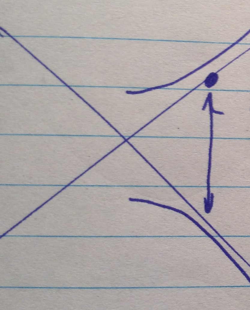
Let’s look for a solution for the \( E + m c^2 > V_0 \) case on the right branch, as sketched in fig. 8.
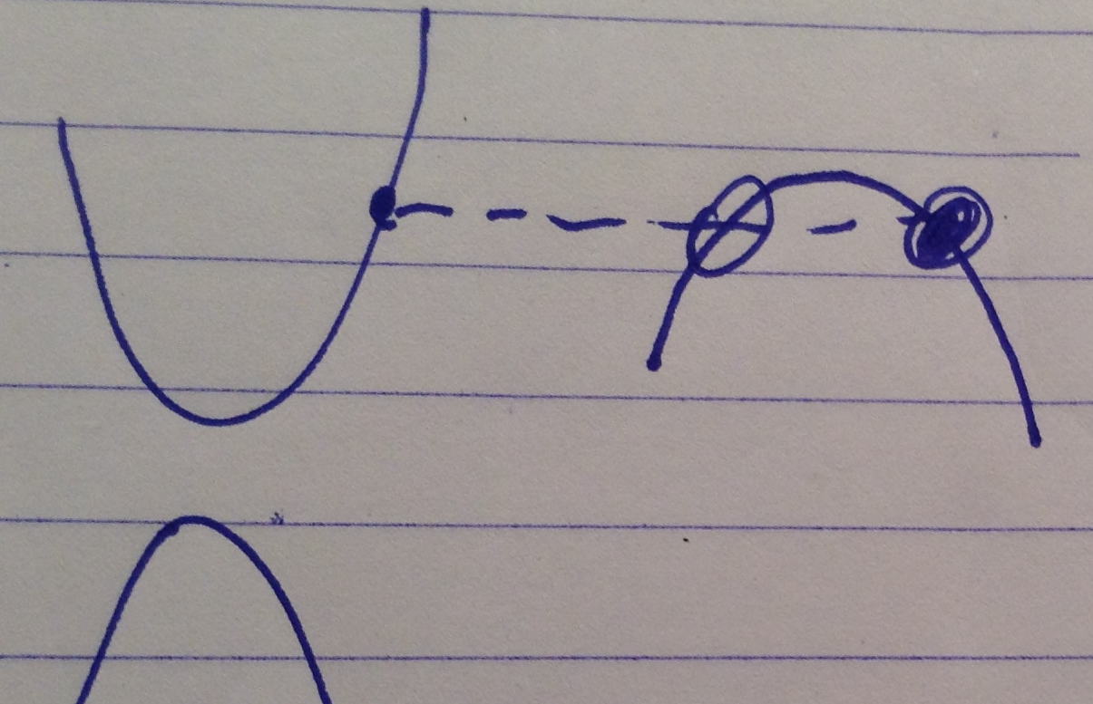
fig. 8. High potential region. Anti-particle transmission.
While the right branch in this case is left going, this might work out since that is an antiparticle. We could try both.
Try
\begin{equation}\label{eqn:qmLecture10:480}
\Psi_{II} = D e^{i k_2 x}
\begin{bmatrix}
-\sin\theta_2 \\
\cos\theta_2
\end{bmatrix}.
\end{equation}
This is justified by
\begin{equation}\label{eqn:qmLecture10:500}
+E \rightarrow
\begin{bmatrix}
\cos\theta \\
\sin\theta
\end{bmatrix},
\end{equation}
so
\begin{equation}\label{eqn:qmLecture10:520}
-E \rightarrow
\begin{bmatrix}
-\sin\theta \\
\cos\theta \\
\end{bmatrix}
\end{equation}
At \( x = 0 \) the exponentials vanish, so equating the waves at that point means
\begin{equation}\label{eqn:qmLecture10:380}
\begin{bmatrix}
\cos\theta_1 \\
\sin\theta_1 \\
\end{bmatrix}
+
\frac{B}{A}
\begin{bmatrix}
\sin\theta_1 \\
\cos\theta_1 \\
\end{bmatrix}
=
\frac{D}{A}
\begin{bmatrix}
-\sin\theta_2 \\
\cos\theta_2
\end{bmatrix}.
\end{equation}
Solving this yields
\begin{equation}\label{eqn:qmLecture10:400}
\frac{B}{A} = – \frac{\cos(\theta_1 – \theta_2)}{\sin(\theta_1 + \theta_2)}.
\end{equation}
This yields
\begin{equation}\label{eqn:qmLecture10:420}
\boxed{
R = \frac{1 + \cos( 2 \theta_1 – 2 \theta_2) }{1 – \cos( 2 \theta_1 – 2 \theta_2)}.
}
\end{equation}
As \( V_0 \rightarrow \infty \) this simplifies to
\begin{equation}\label{eqn:qmLecture10:440}
R = \frac{ E – \sqrt{ E^2 – \lr{ m c^2 }^2 } }{ E + \sqrt{ E^2 – \lr{ m c^2 }^2 } }.
\end{equation}
Filling in the details for these results part of problem set 4.