[Click here for a PDF of this post with nicer formatting]

Disclaimer

Peeter’s lecture notes from class. These may be incoherent and rough.

These are notes for the UofT course ECE1505H, Convex Optimization, taught by Prof. Stark Draper, from [1].

Today

• First and second order conditions for convexity of differentiable functions.
• Consequences of convexity: local and global optimality.
• Properties.

Quasi-convex

$F_1$ and $F_2$ convex implies $\max( F_1, F_2)$ convex.

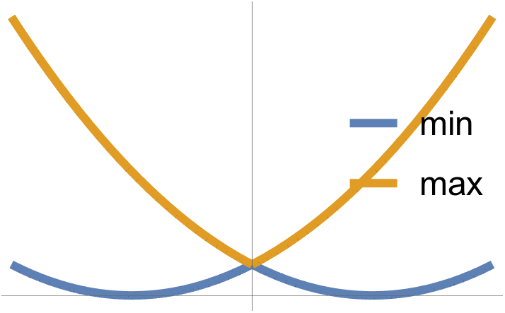
fig. 1. Min and Max

Note that $\min(F_1, F_2)$ is NOT convex.

If $F : \mathbb{R}^n \rightarrow \mathbb{R}$ is convex, then $F( \Bx_0 + t \Bv )$ is convex in $t\,\forall t \in \mathbb{R}, \Bx_0 \in \mathbb{R}^n, \Bv \in \mathbb{R}^n$, provided $\Bx_0 + t \Bv \in \textrm{dom} F$.

Idea: Restrict to a line (line segment) in $\textrm{dom} F$. Take a cross section or slice through $F$ alone the line. If the result is a 1D convex function for all slices, then $F$ is convex.

This is nice since it allows for checking for convexity, and is also nice numerically. Attempting to test a given data set for non-convexity with some random lines can help disprove convexity. However, to show that $F$ is convex it is required to test all possible slices (which isn’t possible numerically, but is in some circumstances possible analytically).

Differentiable (convex) functions

Definition: First order condition.

If

$$\begin{equation*} F : \mathbb{R}^n \rightarrow \mathbb{R} \end{equation*}$$

is differentiable, then $F$ is convex iff $\textrm{dom} F$ is a convex set and $\forall \Bx, \Bx_0 \in \textrm{dom} F$

$$\begin{equation*} F(\Bx) \ge F(\Bx_0) + \lr{\spacegrad F(\Bx_0)}^\T (\Bx – \Bx_0). \end{equation*}$$

This is the first order Taylor expansion. If $n = 1$, this is $F(x) \ge F(x_0) + F'(x_0) ( x – x_0)$.

The first order condition says a convex function \underline{always} lies above its first order approximation, as sketched in fig. 3.

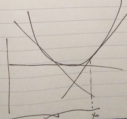
fig. 2. First order approximation lies below convex function

When differentiable, the supporting plane is the tangent plane.

Definition: Second order condition

If $F : \mathbb{R}^n \rightarrow \mathbb{R}$ is twice differentiable, then $F$ is convex iff $\textrm{dom} F$ is a convex set and $\spacegrad^2 F(\Bx) \ge 0 \,\forall \Bx \in \textrm{dom} F$.

The Hessian is always symmetric, but is not necessarily positive. Recall that the Hessian is the matrix of the second order partials $(\spacegrad F)_{ij} = \partial^2 F/(\partial x_i \partial x_j)$.

The scalar case is $F”(x) \ge 0 \, \forall x \in \textrm{dom} F$.

An implication is that if $F$ is convex, then $F(x) \ge F(x_0) + F'(x_0) (x – x_0) \,\forall x, x_0 \in \textrm{dom} F$

Since $F$ is convex, $\textrm{dom} F$ is convex.

Consider any 2 points $x, y \in \textrm{dom} F$, and $\theta \in [0,1]$. Define

$$\begin{equation}\label{eqn:convexOptimizationLecture6:60} z = (1-\theta) x + \theta y \in \textrm{dom} F, \end{equation}$$

then since $\textrm{dom} F$ is convex

$$\begin{equation}\label{eqn:convexOptimizationLecture6:80} F(z) = F( (1-\theta) x + \theta y ) \le (1-\theta) F(x) + \theta F(y ) \end{equation}$$

Reordering

$$\begin{equation}\label{eqn:convexOptimizationLecture6:220} \theta F(x) \ge \theta F(x) + F(z) – F(x), \end{equation}$$

or
$$\begin{equation}\label{eqn:convexOptimizationLecture6:100} F(y) \ge F(x) + \frac{F(x + \theta(y-x)) – F(x)}{\theta}, \end{equation}$$

which is, in the limit,

$$\begin{equation}\label{eqn:convexOptimizationLecture6:120} F(y) \ge F(x) + F'(x) (y – x), \end{equation}$$

completing one direction of the proof.

To prove the other direction, showing that

$$\begin{equation}\label{eqn:convexOptimizationLecture6:140} F(x) \ge F(x_0) + F'(x_0) (x – x_0), \end{equation}$$

implies that $F$ is convex. Take any $x, y \in \textrm{dom} F$ and any $\theta \in [0,1]$. Define

$$\begin{equation}\label{eqn:convexOptimizationLecture6:160} z = \theta x + (1 -\theta) y, \end{equation}$$

which is in $\textrm{dom} F$ by assumption. We want to show that

$$\begin{equation}\label{eqn:convexOptimizationLecture6:180} F(z) \le \theta F(x) + (1-\theta) F(y). \end{equation}$$

By assumption

1. $F(x) \ge F(z) + F'(z) (x – z)$
2. $F(y) \ge F(z) + F'(z) (y – z)$

Compute

$$\begin{equation}\label{eqn:convexOptimizationLecture6:200} \begin{aligned} \theta F(x) + (1-\theta) F(y) &\ge \theta \lr{ F(z) + F'(z) (x – z) } + (1-\theta) \lr{ F(z) + F'(z) (y – z) } \\ &= F(z) + F'(z) \lr{ \theta( x – z) + (1-\theta) (y-z) } \\ &= F(z) + F'(z) \lr{ \theta x + (1-\theta) y – \theta z – (1 -\theta) z } \\ &= F(z) + F'(z) \lr{ \theta x + (1-\theta) y – z} \\ &= F(z) + F'(z) \lr{ z – z} \\ &= F(z). \end{aligned} \end{equation}$$

Proof of the 2nd order case for $n = 1$

Want to prove that if

$$\begin{equation}\label{eqn:convexOptimizationLecture6:240} F : \mathbb{R} \rightarrow \mathbb{R} \end{equation}$$

is a convex function, then $F”(x) \ge 0 \,\forall x \in \textrm{dom} F$.

By the first order conditions $\forall x \ne y \in \textrm{dom} F$

$$\begin{equation}\label{eqn:convexOptimizationLecture6:260} \begin{aligned} F(y) &\ge F(x) + F'(x) (y – x) F(x) &\ge F(y) + F'(y) (x – y) \end{aligned} \end{equation}$$

Can combine and get

$$\begin{equation}\label{eqn:convexOptimizationLecture6:280} F'(x) (y-x) \le F(y) – F(x) \le F'(y)(y-x) \end{equation}$$

Subtract the two derivative terms for

$$\begin{equation}\label{eqn:convexOptimizationLecture6:340} \frac{(F'(y) – F'(x))(y – x)}{(y – x)^2} \ge 0, \end{equation}$$

or
$$\begin{equation}\label{eqn:convexOptimizationLecture6:300} \frac{F'(y) – F'(x)}{y – x} \ge 0. \end{equation}$$

In the limit as $y \rightarrow x$, this is
$$\begin{equation}\label{eqn:convexOptimizationLecture6:320} \boxed{ F”(x) \ge 0 \,\forall x \in \textrm{dom} F. } \end{equation}$$

Now prove the reverse condition:

If $F”(x) \ge 0 \,\forall x \in \textrm{dom} F \subseteq \mathbb{R}$, implies that $F : \mathbb{R} \rightarrow \mathbb{R}$ is convex.

Note that if $F”(x) \ge 0$, then $F'(x)$ is non-decreasing in $x$.

i.e. If $x < y$, where $x, y \in \textrm{dom} F$, then

$$\begin{equation}\label{eqn:convexOptimizationLecture6:360} F'(x) \le F'(y). \end{equation}$$

Consider any $x,y \in \textrm{dom} F$ such that $x < y$, where

$$\begin{equation}\label{eqn:convexOptimizationLecture6:380} F(y) – F(x) = \int_x^y F'(t) dt \ge F'(x) \int_x^y 1 dt = F'(x) (y-x). \end{equation}$$

This tells us that

$$\begin{equation}\label{eqn:convexOptimizationLecture6:400} F(y) \ge F(x) + F'(x)(y – x), \end{equation}$$

which is the first order condition. Similarly consider any $x,y \in \textrm{dom} F$ such that $x < y$, where

$$\begin{equation}\label{eqn:convexOptimizationLecture6:420} F(y) – F(x) = \int_x^y F'(t) dt \le F'(y) \int_x^y 1 dt = F'(y) (y-x). \end{equation}$$

This tells us that

$$\begin{equation}\label{eqn:convexOptimizationLecture6:440} F(x) \ge F(y) + F'(y)(x – y). \end{equation}$$

Vector proof:

$F$ is convex iff $F(\Bx + t \Bv)$ is convex $\forall \Bx,\Bv \in \mathbb{R}^n, t \in \mathbb{R}$, keeping $\Bx + t \Bv \in \textrm{dom} F$.

Let
$$\begin{equation}\label{eqn:convexOptimizationLecture6:460} h(t ; \Bx, \Bv) = F(\Bx + t \Bv) \end{equation}$$

then $h(t)$ satisfies scalar first and second order conditions for all $\Bx, \Bv$.

$$\begin{equation}\label{eqn:convexOptimizationLecture6:480} h(t) = F(\Bx + t \Bv) = F(g(t)), \end{equation}$$

where $g(t) = \Bx + t \Bv$, where

$$\begin{equation}\label{eqn:convexOptimizationLecture6:500} \begin{aligned} F &: \mathbb{R}^n \rightarrow \mathbb{R} \\ g &: \mathbb{R} \rightarrow \mathbb{R}^n. \end{aligned} \end{equation}$$

This is expressing $h(t)$ as a composition of two functions. By the first order condition for scalar functions we know that

$$\begin{equation}\label{eqn:convexOptimizationLecture6:520} h(t) \ge h(0) + h'(0) t. \end{equation}$$

Note that

$$\begin{equation}\label{eqn:convexOptimizationLecture6:540} h(0) = \evalbar{F(\Bx + t \Bv)}{t = 0} = F(\Bx). \end{equation}$$

Let’s figure out what $h'(0)$ is. Recall hat for any $\tilde{F} : \mathbb{R}^n \rightarrow \mathbb{R}^m$

$$\begin{equation}\label{eqn:convexOptimizationLecture6:560} D \tilde{F} \in \mathbb{R}^{m \times n}, \end{equation}$$

and
$$\begin{equation}\label{eqn:convexOptimizationLecture6:580} {D \tilde{F}(\Bx)}_{ij} = \PD{x_j}{\tilde{F_i}(\Bx)} \end{equation}$$

This is one function per row, for $i \in [1,m], j \in [1,n]$. This gives

$$\begin{equation}\label{eqn:convexOptimizationLecture6:600} \begin{aligned} \frac{d}{dt} F(\Bx + \Bv t) &= \frac{d}{dt} F( g(t) ) \\ &= \frac{d}{dt} h(t) \\ &= D h(t) \\ &= D F(g(t)) \cdot D g(t) \end{aligned} \end{equation}$$

The first matrix is in $\mathbb{R}^{1\times n}$ whereas the second is in $\mathbb{R}^{n\times 1}$, since $F : \mathbb{R}^n \rightarrow \mathbb{R}$ and $g : \mathbb{R} \rightarrow \mathbb{R}^n$. This gives

$$\begin{equation}\label{eqn:convexOptimizationLecture6:620} \frac{d}{dt} F(\Bx + \Bv t) = \evalbar{D F(\tilde{\Bx})}{\tilde{\Bx} = g(t)} \cdot D g(t). \end{equation}$$

That first matrix is

$$\begin{equation}\label{eqn:convexOptimizationLecture6:640} \begin{aligned} \evalbar{D F(\tilde{\Bx})}{\tilde{\Bx} = g(t)} &= \evalbar{ \lr{\begin{bmatrix} \PD{\tilde{x}_1}{ F(\tilde{\Bx})} & \PD{\tilde{x}_2}{ F(\tilde{\Bx})} & \cdots \PD{\tilde{x}_n}{ F(\tilde{\Bx})} \end{bmatrix} }}{ \tilde{\Bx} = g(t) = \Bx + t \Bv } \\ &= \evalbar{ \lr{ \spacegrad F(\tilde{\Bx}) }^\T }{ \tilde{\Bx} = g(t) } \\ = \lr{ \spacegrad F(g(t)) }^\T. \end{aligned} \end{equation}$$

The second Jacobian is

$$\begin{equation}\label{eqn:convexOptimizationLecture6:660} D g(t) = D \begin{bmatrix} g_1(t) \\ g_2(t) \\ \vdots \\ g_n(t) \\ \end{bmatrix} = D \begin{bmatrix} x_1 + t v_1 \\ x_2 + t v_2 \\ \vdots \\ x_n + t v_n \\ \end{bmatrix} = \begin{bmatrix} v_1 \\ v_1 \\ \vdots \\ v_n \\ \end{bmatrix} = \Bv. \end{equation}$$

so

$$\begin{equation}\label{eqn:convexOptimizationLecture6:680} h'(t) = D h(t) = \lr{ \spacegrad F(g(t))}^\T \Bv, \end{equation}$$

and
$$\begin{equation}\label{eqn:convexOptimizationLecture6:700} h'(0) = \lr{ \spacegrad F(g(0))}^\T \Bv = \lr{ \spacegrad F(\Bx)}^\T \Bv. \end{equation}$$

Finally

$$\begin{equation}\label{eqn:convexOptimizationLecture6:720} \begin{aligned} F(\Bx + t \Bv) &\ge h(0) + h'(0) t \\ &= F(\Bx) + \lr{ \spacegrad F(\Bx) }^\T (t \Bv) \\ &= F(\Bx) + \innerprod{ \spacegrad F(\Bx) }{ t \Bv}. \end{aligned} \end{equation}$$

Which is true for all $\Bx, \Bx + t \Bv \in \textrm{dom} F$. Note that the quantity $t \Bv$ is a shift.

Epigraph

Recall that if $(\Bx, t) \in \textrm{epi} F$ then $t \ge F(\Bx)$.

$$\begin{equation}\label{eqn:convexOptimizationLecture6:740} t \ge F(\Bx) \ge F(\Bx_0) + \lr{\spacegrad F(\Bx_0) }^\T (\Bx – \Bx_0), \end{equation}$$

or

$$\begin{equation}\label{eqn:convexOptimizationLecture6:760} 0 \ge -(t – F(\Bx_0)) + \lr{\spacegrad F(\Bx_0) }^\T (\Bx – \Bx_0), \end{equation}$$

In block matrix form

$$\begin{equation}\label{eqn:convexOptimizationLecture6:780} 0 \ge \begin{bmatrix} \lr{ \spacegrad F(\Bx_0) }^\T & -1 \end{bmatrix} \begin{bmatrix} \Bx – \Bx_0 \\ t – F(\Bx_0) \end{bmatrix} \end{equation}$$

With $\Bw = \begin{bmatrix} \lr{ \spacegrad F(\Bx_0) }^\T & -1 \end{bmatrix}$, the geometry of the epigraph relation to the half plane is sketched in fig. 3.

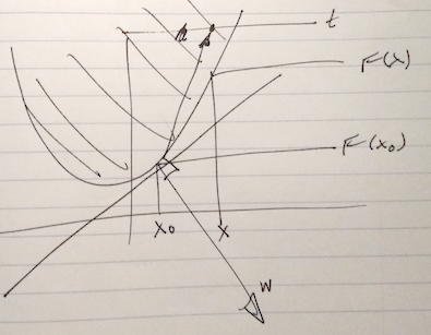
fig. 3. Half planes and epigraph.

References

[1] Stephen Boyd and Lieven Vandenberghe. Convex optimization. Cambridge university press, 2004.